Written by S. Sontum, D. Copeland, and K. Jewett. Edited by R. Sandwick, M. J. Simpson, and R. Bunt

Learning Goals

1. Demonstrate safe handling of hazardous chemicals;
2. Practice writing a hypothesis based on Atomic theory, and write a conclusion based on the hypothesis;
3. Practice using a thistle tube;
4. Generate hydrogen gas and then use it as a reducing agent;
5. Perform chemical degradation analysis, then use the results to calculate an empirical formula;
6. Observe elements that have different states of matter: solid copper, liquid bromine, and gaseous hydrogen;
7. Write a balanced equation to describe a chemical reaction, and draw Lewis structures for reagents involved in the reaction.

Introduction

In the summer of 1803 John Dalton was working on the relative weights of elements that combine in chemical reactions.  He summarized the results of these experiments in his law of multiple proportions: When two or more elements unite to form more than one compound, the masses of one element that combine with a given mass of another are in ratios of small integers.

For example consider the oxides of nitrogen with the formulas N₂O (nitrous oxide or laughing gas), NO (nitric oxide) and NO₂ (nitrogen dioxide).  Because these compounds contain the same element in different proportions they may be used to illustrate the law of multiple proportions. If we use 14 g of nitrogen to make each of these oxides, the mass of oxygen combining with this mass of nitrogen are 8 g in N₂O, 16 g in NO, and 32 g in NO₂.  These numbers 8: 16: 32 are simple fractions of each other, as required by the law.

To explain these experiments Dalton drew up the tenets of his atomic theory.  Is the concept of the atom just a theoretical construct? The atom was not an abstraction to him or to the modern day chemist.  Each indivisible atom has a unique physical weight. The multiple proportion ratios are simply a reflection of the mole ratios or atom ratios given by the molecular formula. There has been debate among historians as to the order of Dalton’s two great generalizations.  Which came first, the atomic theory or the law of multiple proportions? Most probably in Dalton’s mind the two ideas were essentially one, just as these two ideas are now combined in the modern day concept of a molecular formula.

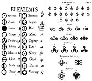
Dalton’s elements  http://thehistoryoftheatom.weebly.com/john-dalton.html

Background

In this experiment you will determine the molecular formula of a metal bromide by first decomposing it with heat, then converting it to a metal oxide by oxidation, and finally reducing it to a pure metal.  Similar steps are used by the mining industry to refine metals. Metals are often found in nature as metal oxide ores. Metal oxides are examples of inorganic salts [Mn+ O2-] where the metal is found as a positive ion ionically bonded to oxygen dianions (oxides).  Formerly, the term oxidation meant “reaction with oxygen” and the term reduction meant “to refine a metal.” Oxidation is now more generally defined as the loss of electrons and reduction is defined as the gain of electrons. Using this definition M2+ is an example of a oxidized metal because it has lost electrons (two) relative to its neutral or elemental form of the metal.  A few metal oxides, such as those of silver and mercury, can be decomposed to free metal by heat alone. All others must react with reducing agents. Reduction results in the removal of oxygen as the positive metal is converted to its neutral or metallic form by gaining electrons. In the preparation of metals from their oxide ores, carbon in the form of coke is often used to reduce the metal because it is relatively inexpensive.  In the laboratory, hydrogen gas is a very convenient reducing agent. At high temperature hydrogen will reduce many metal oxides including copper oxides.

Hydrogen can easily be generated by the oxidation/reduction reaction between zinc metal and sulfuric acid:

Zn(s) + H₂SO₄(aq) —> ZnSO₄(aq) + H₂(g)

You will be given a compound (compound I) that contains only copper and bromine.  When heated, compound 1 loses part of its bromine to form a different compound (compound II), liberating bromine gas in the process:

2 CuBr_x(s) → 2 CuBr_y(s) + (x-y) Br₂(g)

On subsequent treatment with nitric acid all of the residual bromine is removed in a series of oxidation reactions and only an oxide of copper remains.  This series of reactions can be summarized as:

2 CuBr_y(s)  + z O₂(g) → 2 CuO_z(s) + y Br₂(g)

Finally we can determine the mass of copper by reducing the copper oxide to pure metallic copper with hydrogen gas:

CuO_z(s) + z H₂(g) → Cu(s) + z H₂O(g)

From the mass losses accompanying the stepwise removal of bromine, we can calculate how much bromine there was in compound I and compound II.  The relationship between these masses and the mass of copper in the sample will allow us to demonstrate the law of multiple proportions.

Procedure

Note: Perform this lab with a partner.

Part I: Transformation of Compound I to Compound II

1. Determine precisely on an analytical balance the mass of your large Pyrex test tube. Then add about a gram of compound I, and reweigh the tube and contents. Note the color of compound I. Record this data in Table 1.
2. In the hood, assemble the apparatus shown in Figure 1. The test tube is slightly inclined to keep the sample away from the rubber stopper. The Florence flask is filled about half full of water and serves to trap the noxious bromine vapor that will be formed. Tap a spatula tip full of sodium thiosulfate to the water. Have your laboratory instructor or TA check the apparatus before proceeding. Note: Bromine is a poisonous oxidizing agent. Avoid inhaling the vapor. Keep the liquid off your skin. Any spillage should be treated immediately with sodium thiosulfate and lots of water.
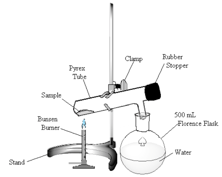
3. 

   Figure 1

   Heat the sample gently. If bromine (a dark-red liquid) condenses at the upper end of the test tube, warm it gently to vaporize the liquid. Continue to heat the sample until no more bromine vapor is evolved (bromine vapor is yellow), perhaps 10 minutes.

4. Allow the test tube to cool. Remove the stopper, and “pour” any residual bromine gas into the Florence flask. Clean out any rubber stopper residue.
5. Remove the test tube from the hood. If you notice a strong smell similar to chlorine, immediately put the test tube back into the hood and attempt to pour out more residual bromine.
6. Weigh the tube and contents precisely and note the color of compound II. Record this data in Table 1.

Part II: Transformation of Compound II to Copper Oxide

1. Working in the hood, pour about 1.5 mL of concentrated nitric acid into the test tube containing compound II. Note: Nitric acid is extremely corrosive to the skin.  Flush immediately with large amounts of water in case of contact with your skin.
2. Reassemble the apparatus of Figure 1.
3. Heat gently to avoid spattering until the dry blue-green copper nitrate is formed and then heat strongly to form the black copper oxide. Wave the flame up and down the tube until the yellow vapor disappears. If the copper oxide is not completely dry, heat until it appears dry. You can’t overdo this step, so really let it burn a long time, perhaps 15 minutes. Let it cool, then clean out any rubber stopper residue.
4. Remove the test tube from the hood. If you notice a strong smell similar to chlorine, immediately put the test tube back into the hood and attempt to pour out more residual bromine.
5. Weigh the black copper oxide and test tube. Record this data in Table 1.
6. Clean up: the bromine and sodium thiosulfate solution can go down the drain. Keep your copper oxide.

Part III: Reduction of Copper Oxide to metallic Copper

Assemble the apparatus shown in Figure 2. Note: be very careful to use the following method for introducing glass connections into rubber stoppers or rubber connectors (very severe cuts can result if the glass tubing breaks and the jagged ends get pushed into the hands): moisten the stopper and tube with a small amount of water or glycerol for lubrication.  Grasp stopper and tube close together with a cloth, and insert the tube into the stopper with a twisting motion, being careful and applying pressure gently.

• Place about 20 g of a combination of granulated and pieces of zinc in the Erlenmeyer flask.  Be sure to have the bottom of the thistle tube extending to the bottom of the flask (check that the tube is not blocked by the zinc).
• Fill the calcium chloride tube two-thirds full of anhydrous calcium chloride.
• Being careful that all of the copper oxide stays toward the closed end of the test tube, attach the tube to your apparatus.  Tilt the test tube slightly upward at the closed end. The gas jet is a short piece of red tubing connecting the side-arm on your test tube and the glass portion of a medicine dropper.
• Make a Pyrex tube approximately 20 cm long fire-polished at both ends to place in the test tube.
• Make sure that all connections are tight.  Leave enough space between the ends of the glass tubes in the rubber connector so that the connector can be pinched shut.
  

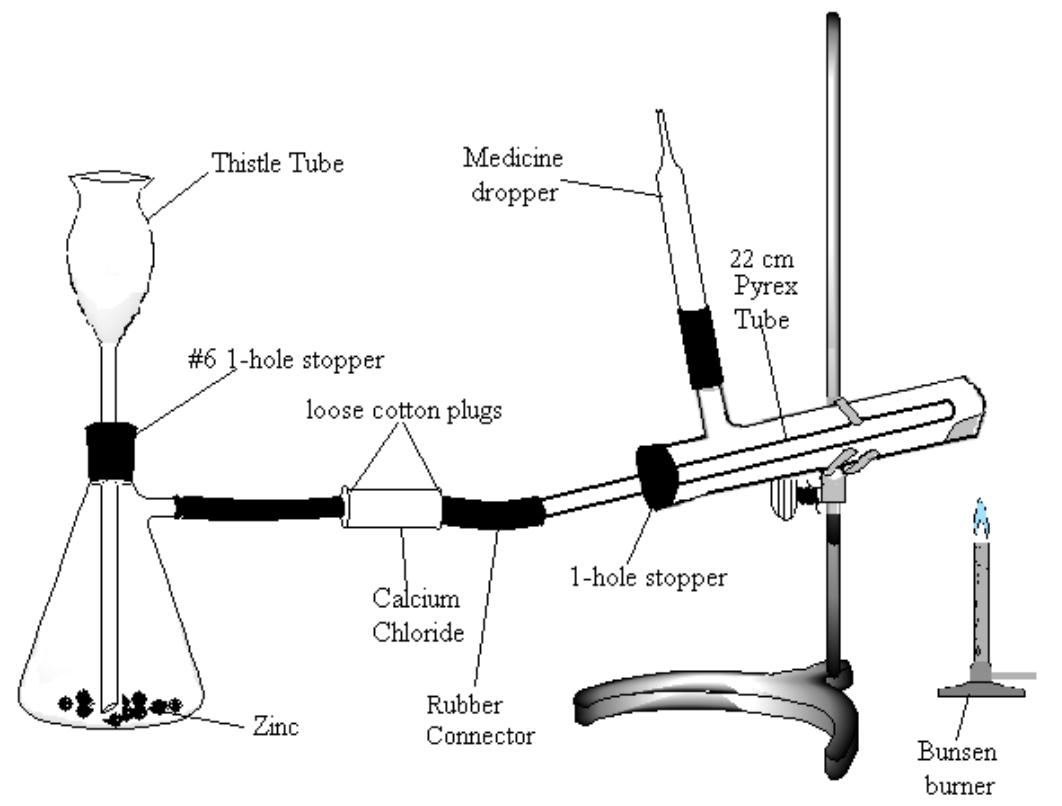
  Figure 2

1. Introduce 1.0 mL of a dilute solution (0.2 M) of copper sulfate and then 10 mL of water into the generator through the thistle tube.
2. Add 30 mL of dilute (6 M) sulfuric acid. Make sure the bottom of the thistle tube is below the surface of the liquid. Add more acid if it is too shallow.
3. Bubbles of hydrogen will form and sweep through the apparatus, flushing out the air. A mixture of hydrogen and air is very explosive, and if the gas escaping from the delivery tube is lighted before all of the air has been driven out of the generator, a violent explosion will result. To avoid this danger, the gas issuing from the delivery tube of a hydrogen generator should always be lighted in the following manner:  Invert a test tube over the jet and allow it to fill with gas.  Close the end of the test tube with the thumb and, bringing the inverted test tube near a Bunsen flame which is at least 2 ft from the generator, remove the thumb and light the gas.  Then, holding the tube still in the inverted position, immediately attempt to light the gas coming from the delivery tube with the nearly invisible flame issuing from the test tube.  If the gas in the generator is explosive, it will explode in the test tube and leave no flame.  When, however, the flame in the tube lasts long enough to enable one to light the gas issuing from the jet, it is evident that the gas in the generator is no longer explosive.
4. After the hydrogen at the jet has been lighted, hold the burner in the hand and gently heat the end of the test tube containing the oxide. Gradually raise the temperature to red heat. (However be careful that you do not melt your test tube!) It is safe to proceed with the experiment even if the hydrogen flame goes out, provided a brisk and steady evolution of hydrogen is maintained. It may be necessary to add more sulfuric acid to the bottle.  If the level of the acid is below the bottom of the thistle tube, pinch the rubber tubing to raise the level of the acid, thus preventing air from being trapped in the thistle tube.  Why is this dangerous?
5. Continue the heating until all of the oxide has been converted to metal.  (Caution!  The tube gets very hot.) This will require about 10 – 15 minutes.  What is the product which collects in the cooler portion of the test tube?
6. Allow the tube to cool in the current of hydrogen, pinch the rubber connector for a moment to put out the hydrogen flame, and disconnect the apparatus.  Wipe out any water or rubber stopper residue you find at the mouth of the test tube with a paper towel, and weigh the tube. Record the data in Table 1.
7. Clean up: copper dust goes in the trash can. Decant the water off of the leftover zinc. Pour this water down the drain. Put wet zinc in the collection beaker for reuse.

Report

Fill out this worksheet. Turn in either a paper or digital copy.

Learning Goals

1. Practice using an analytical balance;
2. Practice using a graduated cylinder;
3. Apply significant figures rules to experimental calculations;
4. Perform linear regression.

Introduction

Dmitri Mendeleev

When Dmitri Mendeleev published the first periodic table, he arranged the elements to illustrate their periodic trends. Many elements that we know of today had not been discovered yet (Note: scientists continue to discover new elements today), so Mendeleev left gaps where there seemed to be discontinuities in the trends. One of these gaps was an element that seemed to be missing from group 14 between silicon and tin. He called the missing element “eka-silicon.”

Clemens Winkler discovered a new element in 1886. Its physical properties were similar to antimony and arsenic, but its chemical reactivity fit with elements in group 14, so it wasn’t clear where the new element fit on the periodic table. Finally, Winkler determined the atomic mass of the new element, which matched Mendeleev’s prediction for eka-silicon, so the element was placed in group 14 and named “Germanium” after his homeland of Germany.

https://en.wikipedia.org/wiki/Germanium

In this experiment, you will measure the density of 3 of the elements in group 14 and predict the density of Germanium.

Background

Density is defined as mass per volume. It is normally expressed in units of g/cm³ or g/mL (these are equivalent). Therefore, to measure the density of these elements, you will need to measure both the mass and the volume.

Measuring the mass is easy: we have highly accurate analytical balances. They are calibrated on a regular basis. Measuring the volume is a little trickier and requires careful attention to significant figures.

Procedure

Note: this lab is performed individually, but you will need to collaborate with two other students to complete the data analysis. Each student in your group of three will measure the density of one of the elements provided, and you will combine your results to predict the density of germanium. You may need to provide data for more than one group, depending on how many students are in your lab section.

Measurement of the density of a group 4 element

1. Obtain a sample of your element: For tin or silicon, use approximately 10 g. For lead, use approximately 25 g. Tare your weighing vessel. This could be a weigh boat or a small beaker. Place the sample in the vessel. Record the exact mass, including all of the decimal places displayed on the balance, in Table 2. Pro-tip: when you tare a weighing vessel, you are subtracting the mass of the weighing vessel from the mass of whatever you are weighing. Scientists normally use the balance to do this subtraction automatically by setting the mass of the empty weigh vessel to zero immediately before using the balance. 
2. Put approximately 15 mL of DI H2O (“deionized water”) into a 25-mL graduated cylinder. DI H2O is found in the small white faucets in every sink. Record the exact volume to the nearest 0.02 or 0.05 mL in Table 2. If you cylinder has graduation lines representing 0.2 mL, then estimate to 0.02 mL. If it has graduation lines representing 0.5 mL, then estimate to 0.05 mL. Ask your instructor or TA if you’re not sure how to figure this out.
3. Place the element sample carefully into the graduated cylinder. Make sure you don’t splash any water. Record the volume of the water and the sample to the nearest 0.02 or 0.05 mL in Table 2. Precision should match your previous measurement in step 2.
4. Dry the sample and return it.

Data analysis

1. Use your data from Table 2 to calculate the density of your sample. Record the density in Table 3.
2. Obtain the densities of the two other elements from two other students. Fill in  Table 3.
3. Use Excel or some other plotting software to plot the densities of each element as a function of period number on the periodic table (eg. Silicon would be 3, tin would be 5, etc.). If you are unfamiliar with plotting in Excel and linear regression, refer to the Excel lab techniques page or consult the CTLR. Here is an example of linear regression using Google Sheets.
4. Perform linear regression. Find the equation for a line that takes the period number and outputs a density for elements in group 14.
5. Input germanium’s period number (4) and solve for the predicted density of germanium.
6. Calculate the percent error for the predicted density of germanium compared to the literature density of germanium. Percent error is the absolute value difference between your experimental value and the literature value, divided by the literature value, multiplied by 100.

Report

Fill out this worksheet. Turn in either a paper or digital copy. Attach your graphs.

Note: Plan on dressing in old clothes for this lab. These dyes are powerful and may permanently stain your clothes if you splash or drip them on yourself.

Part 1: Prepare cotton for tie dye

(Hint: If you read through these instructions before coming to lab, plan on completing this step before the pre-lab discussion to ensure the most vibrant colors possible.)

1. Use a permanent marker to write your name on the tag of your garment.
2. Soak your garment in the sodium carbonate wash for at least 30 minutes. This solution is very basic, so wear gloves when in contact with the wash.

Part 2: Tie and dye cotton

1. Wring out the garment to dry it as much as you can.
2. Fold and tie with waxed sinew your garment however you like.  Here are some designs you might like to try.
   
3. Working in a foil pie pan on a surface covered in newspaper, apply the dye. Use your knowledge of the color wheel to select colors that will mix well. (Hint: colors that are next to each other on the color wheel mix well, but colors across from each other make brown/black.) Be sure to saturate the fabric with dye, but don’t put so much on that the dye pools underneath the fabric. Again, wear gloves when working with dye or it will dye your skin!
4. Wrap your garment in clean newspaper and put it in a sealed plastic bag. Place it in your cabinet and leave it there for the week.
5. Clean your foil pie pan, return it, and throw away wet newspaper.

Part 3: Rinse loose dyes from your tie dye

1. Wearing gloves, snip the sinew with scissors and untie your garment. Throw away the wet newspaper and sinew.
2. Rinse the garment with cool water until no more dye comes off the garment. This will probably take 5-10 minutes.
3. Put the shirt back into the plastic bag and give it to the instructor.

Learning Goals

1. Construct hybrid molecular orbital diagrams and connect this theory with properties of molecules;
2. Perform computational chemistry calculations to form a theoretical basis for an experiment;
3. Prepare solutions via serial dilutions;
4. Explore limitations in measurements made with the spectrophotometer and analytical, including the differences between absorbance measurements and percent transmittance measurements;

Introduction

The sun emits a continuous spectrum of ultraviolet (UV), visible, and infrared light. Of particular concern is UV light, which the World Health Organization classifies ultraviolet (UV) light as a known carcinogen. This means that UV light causes cancer. UV light also causes erythema, commonly known as a sunburn, and damages skin fibers, evidenced by wrinkled and sagging skin. 

The Food and Drug Administration (FDA) regulates sunscreen products claiming to protect skin from the sun and assigns a numerical sun protection factor (SPF). The FDA currently requires in vivo testing to measure the SPF; this involves application of the sunscreen to a patch of a volunteer’s skin and then exposing the volunteer to a controlled UV light source until the skin develops a sunburn. The SPF is calculated by comparing the amount of time it takes to sunburn the skin with the sunscreen to the amount of time it takes to sunburn the skin without sunscreen. SPF 15 means it takes 15 times longer to burn the skin with sunscreen than the skin without sunscreen. Unfortunately, this testing requires that a human volunteer gets a sunburn, which increases their risk of skin cancer. The goal of this lab is to develop a laboratory-based scale to measure the SPF without harming human volunteers. Instead of measuring how well a sunscreen protects against sunburn in a human volunteer, you will measure how well a sunscreen blocks UV light in the laboratory using spectrophotometry.

Background

Most sunscreen products block UV light either by absorbing UV or reflecting UV. Mineral-based sunscreens such as titanium dioxide or zinc oxide mostly reflect UV, and organic molecules mostly absorb UV. In this lab, we are using a line of organic-based sunscreens that all have avobenzone as the primary active ingredient. Below is a line diagram of avobenzone. You can see that it exists in two isomer forms, which are called tautomers in this case. One tautomer absorbs UV-A (320 – 400 nm), and one absorbs UV-C (100 – 280 nm). Although the higher energy UV-C is very dangerous in theory, it is absorbed by just about everything, and as a result, unable to penetrate the skin. It is the lower energy UV-A that we need sunscreen to absorb.

Avobenzone tautomeric forms. Top is the keto form, and middle and bottom are enol form. Note that the dashed line connecting the oxygen and hydrogen indicates hydrogen-bonding. Jü (https://commons.wikimedia.org/wiki/File:Avobenzone_Tautomeric_Forms_V1.svg), https://creativecommons.org/licenses/by-sa/4.0/legalcode

Avobenzone, like other organic molecules, can absorb a photon of light energy when an electron moves from a ground state, filled orbital to an excited state, unfilled orbital. The energy difference (ΔE) between the filled and unfilled orbitals is inversely related to the wavelength (λ) of light that can cause that transition.

ΔE = hc / λ

Molecular orbital diagrams predict the electron configuration in a molecule and can explain qualitative differences between molecules. In this lab, you will use molecular orbital theory to decide which tautomer of avobenzone absorbs UV-A and which absorbs UV-C. To verify your prediction, you will use Chem3D Pro molecular modeling software to calculate the wavelength of the absorptions. Note that these predictions are approximate and do not account for solvent effects.

Finally, you will measure the amount of light absorbed by the sunscreen samples at the wavelength that you calculate with the modeling software. A UV-Vis spectrometer will allow you to measure the amount of light absorbed at a given wavelength. Transmittance is a direct measurement of the fraction of the light that the sample blocks. (Note: transmittance doesn’t differentiate between a sample that blocks the light via absorption such as an organic sunscreen and a sample that blocks the light via reflection or scattering such as a mineral sunscreen. This is a source of uncertainty when making measurements on potentially scattering or reflecting samples).

Percent transmittance (% T) = Amount of light that passes through the sample / Amount of light applied to the sample x 100

You may expect percent transmittance to be proportional to the amount of sample present, but surprisingly, it is not. Consult with this webpage for a more complete explanation. Absorbance (A) is Log(1/%T), and this is proportional to the concentration of the chemical you are measuring. The Beer-Lambert law states:

A = ε b c,

where ε is a constant (“molar absorptivity”), b is the length of the sample where the light passes through, and c is the concentration of the sample. Since we are not measuring the concentration of the avobenzone, you will not need to use the Beer-Lambert law, but it may prove useful in future labs. Our spectrophotometers can measure either A or % T.

Procedure

Note: perform this lab with a partner.

Part I: Molecular Orbital Theory Prediction of Active Form of Avobenzone

Follow the instructions on the lab worksheet to create hybridized molecular orbital diagrams for the bond between two carbons in each form of avobenzone.

Part II: Molecular Modeling Calculation of the Peak Absorbance of Avobenzone

1. Open Chem3D 15.1
2. Click on the white panel to the right of the main window. It is titled “ChemDraw-LiveLink.”
3. In the text bar, type “Avobenzone,” then hit “enter.” The keto form of avobenzone should appear.
4. Optimize the structure by hitting “control-m.”
5. There are several things you can do to get a better look at the molecule.
   • You can click the third button from the left on the top toolbar to rotate the molecule. It looks like a circle with an arrow on it. After you click it, you can use the mouse to rotate the molecule.
   • You can click “View” on the main menu, then click “Model Display.” This will present you with many options to change the display of the molecule. For example, “Display Mode” gives you more modes. The “Ball & Stick” mode is most common, but “Wire Frame” is convenient for a very complicated molecule, and “Space Filling” is helpful for visualizing atom size differences.
6. After making the model and optimizing the structure, click “Surfaces” on the main menu, then “Choose Surface,” then “Molecular Orbital.”
   • The HOMO (highest occupied molecular orbital) will automatically be shown, but you can choose another molecular orbital from “Select Molecular Orbital.” You will also see the energies associated with each orbital. The labels are with respect to the HOMO and the LUMO (lowest unoccupied molecular orbital). Notice that the HOMO energy is usually negative, indicating a favorable state, but the LUMO energy is usually positive, indicating an unfavorable state (which is why it is UNOCCUPIED!)
   • The difference between the HOMO and the LUMO energies is the number you want to record; it usually corresponds to the strongest, lowest energy electronic absorption possible for the molecule. ChemDraw reports the the molecular orbital energies in terms of eV, so you will need to convert from those energy units to wavelength units in your post-lab.
7. You will have to switch from the keto form to the enol form manually. Use the tools associated with the “ChemDraw-LiveLink” panel to edit the molecule.
   • You will need to add a bond between two carbons and delete a bond between a carbon and an oxygen. There are two possible configurations of the enol form, but it doesn’t much matter which one you make. The answers you get are almost exactly the same either way.
   • The last step to form the enol is pretty tricky.
     • You have to get a “dummy bond” and attach the double-bonded oxygen to the hydrogen that’s attached to the single-bonded oxygen.
     • Then, optimize the energy via “control-m.”
     • Then, delete that dummy bond before continuing with the procedure to find the HOMO-LUMO energy difference for the enol form (repeating step 6).

Part III: Absorption Spectroscopy of Sunscreens

Note: each group can have only 2 50-mL volumetric flasks. They will be used several times throughout this procedure. Be sure to rinse thoroughly between uses.

Blank the spectrophotometer

1. Prepare a blank cuvette: pour approximately 2 mL of propanol into a cuvette. Label the sample “blank”.
2. Set the spectrophotometer to measure at 357 nm. This should be pretty close to the wavelength you calculated in the modeling section of this experiment (within +/-20 nm). Set the spectrophotometer to measure percent transmittance.
3. Load the “blank” sample into the spectrophotometer in the slot marked “B.” Leave the blank in the B slot for the entire experiment. Hit “measure blank.” This should cause the percent transmittance measurement to say something very close to 100.0%. Ask your instructor or TA if it does not read something between 99.0 and 100.5%. Watch this number for a couple of minutes to ensure your spectrophotometer is giving you a stable reading. If the reading drifts outside of the 99.0 – 100.5% range during a 5 minute period, you will need to let the machine warm up some more. Record the %T measurement for the blank in Table 2.

Measure %T for SPF 4, 8, 15, and 30 Samples

1. Working with one sunscreen solution at a time, transfer about 2 mL of the solution into a cuvette.
2. Put the cuvette into the spectrometer and take the %T measurement immediately. Record the measurement in Table 2.
3. Repeat steps 1 and 2 for each sunscreen sample (SPF 4, 8, 15, 30). If necessary, re-blank the instrument between samples.
4. Also record the masses associated with each sample in Table 1. This information is written on the bottles or the blackboard.

Prepare the SPF 50 sample fresh so you can explore how the sunscreen degrades through light exposure

1. Tare a 50 mL volumetric flask.
2. Use a wooden dowel to transfer a small glob of sunscreen from the tube to the volumetric flask.
3. Record the mass in Table 1. It should be around 0.0250 g. If it is too much, just use the dowel to scrape some out.
4. Fill the flask up to the line with propanol, cap, and shake vigorously. Scrape down the sides of the flask and resume shaking if you need to.
5. Use a 10 mL graduated cylinder to remove 10.00 mL of the solution. Pour the rest of the flask down the drain. Put the 10 mL back into the flask and then fill to the line with propanol. Again, cap and shake vigorously.
6. Immediately begin making measurements with the Genesys 30.

SPF 50 measurements

1. Blank the Genesys 30 spectrophotometer at 357 nm with a cuvette filled with approximately 2 mL of pure propanol.
2. Take out the blank and put in the SPF 50 sample. Record the initial %T in Table 2.
3. Continue taking percent transmittance reading every minute for 10 minutes, recording the data in Table 3. Also write the initial %T in Table 3.

Part IV: Data Analysis

Normalization of Transmittance Measurements to Account for Various Drop Sizes

The first part of your data analysis will be normalizing the transmittance measurements according to the mass of the drop of sunscreen. The equation you will use to normalize the percent transmittance is somewhat complicated and unnecessary for you to derive on your own, but here are the details for those of you who are curious:

The exact amount of sunscreen that you used, the drop size, is directly proportional to the concentration (c) of sunscreen that you produce in the dilution procedure. According to the Beer-Lambert Law, the concentration of the absorbing chemical is directly proportional to the absorbance (A) of the chemical in solution. Absorbance is defined as Log(1/%T), where %T is the percent transmittance, so if you rearrange these expressions algebraically, then you see that %T is proportional to 1/10^c. To normalize for concentration, you will divide your measured %T by 1/10^c. This form is the most simplified form, which you should use to solve for Tables 4 and 5.

Normalized %T = measured %T × 10^c
where c is the mass of the drop, which you recorded in Table 1.

Of course, the blank had no sunscreen, so you will not need to normalize its %T.

Graphing Data and Linear Regression Fits

You will be making 2 graphs. Your graphs must all have titles, axis labels, axis units (if applicable), and a labeled legend. The legend should display the equation of the line of best fit and the R² value. You can use Excel, Google Sheets, or any graphing software that you are comfortable with. I recommend Google Sheets if you are working very closely with a partner, but Excel is generally easier to use.

1. Graph SPF vs the concentration-normalized initial percent transmittance (data in Table 4). Fit the data with a line.
2. Graph time (in minutes) vs the concentration-normalized percent transmittance for SPF 50 (data in Table 5). Fit the data with a line.

Report

Fill out this worksheet. Turn in either a paper or digital copy.

Learning Goals

1. Use bomb calorimetry to measure heat of reaction;
2. Use a thermometer and analyze the limitations of thermometry;
3. Observe changes in phases of matter and consider the challenges associated with volatile substances;
4. Apply the ideal gas law and analyze the limitations of using the ideal gas law in an experiment;
5. Synthesize a simple procedure and a data table to collect experimental data;
6. Choose a follow-up experiment based on initial results;
7. Write a conclusion based on a specific prompt and tabulate results to support the conclusion.

Ideas for portions of this lab were drawn from the University of Pennsylvania Laboratory Program for Chem 53, accessed at this webpage: http://www.sas.upenn.edu/~kennethp/chemlab1.pdf, and the University of Calgary Laboratory Program for Organic Chemistry, accessed at this webpage: http://www.chem.ucalgary.ca/courses/351/laboratory/boilingpoint.pdf.

Introduction

https://qph.ec.quoracdn.net/main-qimg-4161e9231033aa335aca697a3ef0c4e2

In many ways, chemistry can be a puzzle: since you cannot see atoms directly, you must instead collect as many pieces of data as you can and put them together to get the best possible answer. In this lab, you are tasked with identifying an unknown volatile liquid.

First, you will measure the molar mass of the liquid using the ideal gas law, but is the molar mass enough information to identify an unknown? How much uncertainty is associated with the molar mass measurement, anyway? If you were publishing a paper and wanted to convince the scientific community that you have identified a liquid, measuring the molar mass would surely not be enough information!

As additional pieces of evidence, you will measure the density in the liquid state, the boiling point, and the heat of combustion. These four pieces of evidence should pinpoint the exact identity of the liquid with enough certainty to convince even the most skeptical audience, who is hopefully yourself.

When you think you know the identity of the unknown, you can run a confirmatory test.

Background

What is a volatile liquid?

A volatile liquid is a liquid that vaporizes readily under normal conditions. Many volatile liquids have a noticeable smell because they vaporize into your nose! Throughout this lab, you will be working with a volatile liquid. When it is warm, it is mostly a gas, and when it is cool it is mostly a liquid. Note that you will be measuring the density of the substance in both the liquid and the gaseous state, but you will find that the tendency of the volatile liquid to vaporize and condense introduces uncertainty in both of these measurements.

Measuring molar mass from density of the gaseous state

The ideal gas law provides a way to relate the number of moles of a gas to the volume of the gas: n/V = P/RT

If you are also able to relate the number of grams of the gas to the volume of the gas (g/L, in other words, density), then these two formulas together allow you to then relate the number of grams of the gas and the moles of the gas, which is the molar mass: molar mass = (density)RT / P.

Your textbook shows a more detailed derivation in Section 8.3.

In this lab, you will measure the density of a volatile liquid in its gaseous state, the pressure, and the temperature, and this will allow you to calculate the molar mass. To measure the density, you will need to measure the mass and volume of a gas. The procedure will guide you through forming the gas and measuring the mass, but you must design your own method of measuring the volume of the gas. Be creative! Try to get as many significant figures as possible.

Heat of combustion

This is a topic you have not yet covered, but you will soon! Here is a simple explanation of what you need to know for this lab:

The heat of combustion is the amount of energy released when a given amount of a substance is burned in the presence of excess oxygen. Normally this value is reported in terms of energy per mole of the substance, but because we do not yet know the molar mass of the liquid, we will measure it in terms of energy per gram of the substance and compare it to the list of possible sample identities at the bottom of this page, also in those units, in order to identify the liquid.

Density of the liquid state

You should be very comfortable measuring the density of a liquid. You just need the mass and the volume: density = mass/volume. You will be comparing the density of your liquid to the list of possible sample identities at the bottom of this page to help you identify the liquid.

Refer back to Lab 1 for a refresher on density measurements.

Boiling point

Boiling point is the temperature at which a substance changes from a liquid state to a gaseous state. Boiling point is actually a function of pressure, but because most people measure it under atmospheric pressure, it is typically reported at 1.000 atm (1013 mbar). If you notice that the atmospheric pressure on the day of your measurement is greater than or less than 1013 mbar, know that this will contribute to a discrepancy between your results and the literature boiling point values.

Procedure

Note: do this lab with a partner. There are five parts to this lab, which will be done over two weeks. I suggest doing part 1 on the first week and parts 2-5 on the second week, although you may chose to do parts 2 and 3 whenever it is convenient. Be sure to use the same thermometer throughout the experiment.

1. Measuring molar mass from density

Thermometer calibration

At some point, you probably had this thought but were afraid to say it out loud: “are these thermometers right? I always thought water boiled at 100 °C, but it looks like this water is boiling at 105 °C. I don’t know, maybe I’m reading it wrong?” If you have had this thought, then pat yourself on the back for being observant. The alcohol thermometers are not perfect, and to get a reasonably accurate temperature measurement with them, you will need to calibrate them. Since we are making most of our temperature measurements in this experiment near 100 °C, we will calibrate at 100 °C.

Bring a beaker of tap water to a rolling boil over a bunsen burner. It doesn’t matter what size beaker and exactly how much water, but a 600 mL beaker about 3/4 filled with tap water would be a great choice. Once boiling, place your thermometer into the water. Hold it or clamp it so it doesn’t touch the bottom or sides. When the temperature is stable, record the “thermometer calibration temperature” to the nearest 0.2 °C in Table 1.

You can now calculate the offset for your individual thermometer.

100.0°C – “thermometer calibration temperature”(°C) = thermometer offset (°C)

This number may be positive or negative. Use a piece of label tape to label your thermometer with its thermometer offset. From now on, factor that offset into your temperature measurements before recording them in your data table. Keep that calculator handy!

As an example, let’s say your thermometer calibration temperature is 105.0 °C.

100.0°C – 105.0 °C = -5.0 °C

Now you know to subtract 5.0 °C from every temperature you measure throughout the experiment. If your thermometer reads 92.2 °C, then record 92.2 °C – 5.0 °C = 87.2 °C.

Pressure

Record the barometric pressure of the atmosphere in Table 1. If you have reason to believe the pressure is changing throughout the experiment (maybe there is a hurricane outside?), check it before beginning every trial, but normally checking at the beginning of the experiment is sufficient.

Mass and temperature

Use the same 125-mL Erlenmeyer flask throughout this section. Dry the Erlenmeyer flask thoroughly. Measure the mass of the 125-mL Erlenmeyer flask with an Aluminum foil cover secured with a rubber band. Trim the Aluminum foil cover to right below the rubber band. Record the mass of the covered flask in Table 1. Make a tiny hole in the foil cover with a thumbtack.

Set up a hot water bath with a 600 mL beaker about 3/4 filled with tap water, similar to the one shown:

Bring the water to a boil over a blue bunsen flame.

While the water begins to heat, remove the foil cover and rubber band, place about 2 mL of the volatile liquid from the small bottle into the Erlenmeyer flask, then replace the foil cover and rubber band.

Turn off the flame. Submerge the covered Erlenmeyer flask up to its neck in the hot water, and use a clamp to attach it to the ring stand. Add more water if you need it to cover the flask up to the neck, but try not to get the aluminum foil wet.

Also, submerge a thermometer in the water, and use a clamp to attach it to the ring stand.

Monitor the temperature of the water to ensure it stays around 90 °C (don’t forget to factor in your calibration offset). Turn on the flame if the temperature drops below 80 °C. Maintaining this temperature, watch the vapor escape through the pinhole. Watch for the vapor to stop escaping through the pinhole and for visible condensation in the flask to disappear (tendrils dripping down the sides of the inside of the flask). This should take no more than 10 minutes. If you continue seeing condensation after the first 10 minutes, turn up the heat because your thermometer may be reading low. You can verify that the vapor has stopped escaping by holding a small watch glass over the pinhole and seeing that no condensation develops right above the pinhole. As soon as the vapor stops, record the temperature of the hot water bath to the nearest 0.2 °C in Table 1. Be sure to factor in the calibration offset!

Remove the Erlenmeyer flask from the hot water bath, but keep the cover on. Be sure all of the liquid has vaporized. If there is visible liquid, put it back into the hot water bath for a few minutes. Dry the outside of the flask completely. Then, measure the mass of the covered flask with the vapor inside (it may condense back to a liquid). If the mass is not stable, let it cool longer. Record the mass in Table 1. Expect a mass around 0.2 g. Consider re-doing the trial if your mass is much lower or higher.

Repeat this procedure two more times for a total of 3 trials. You may reuse your hot water bath. You must use the same 125-mL Erlenmeyer flask every time, but make sure you dump out the gas and any condensation before weighing the flask empty. If your aluminum foil gets wet, then you should use a new piece.

Volume

Measure the volume of your Erlenmeyer flask using your method, your partner’s method, or a combination of the two. If you need to measure the mass of the water in the flask, be sure to use a high capacity balance such as the CPA324s, which measures up to 320 g. Try not to spill water on the balances. Be sure to clean it up if you do. Record your data in Table 2.

2. Heat of combustion

When it is your turn to use the bomb calorimeter, begin by preparing your sample for analysis:

The experimental sample – this is a clean sample cup with 1.00 g of the volatile liquid inside. Record the exact mass of the volatile liquid in a tared sample cup in Table 3. Cover the sample cup with a piece of parafilm immediately after recording the mass of the sample to ensure none of the sample evaporates.

Your instructor or TA will walk you through measuring the heat of combustion for the sample. You will need the mass of the liquid in order to operate the bomb calorimeter. Record your results in Table 3.

3. Density of liquid state

Use a clean, dry 100 mL volumetric flask with a ground glass stopper for this experiment. How many significant figures do you get? Ask if you are not sure.

Measure the mass of the empty volumetric flask and stopper. Record the data in Table 4.

Fill the volumetric flask exactly to the point where the bottom of the meniscus is on the ground line with the volatile liquid from the bottle labeled “use for density of liquid experiment.” Cover the flask immediately to ensure none of the liquid escapes.

Measure the mass of the filled volumetric flask and stopper. Record the data in Table 4.

4. Boiling point

I will provide a demonstration apparatus for this rather complex set-up, but this is a description of how to build it:

Use the same thermometer that you previously calibrated. If you aren’t sure it is the same one, repeat the calibration procedure and record the offset. Gently push a thermometer through a split rubber stopper. Push the stopper up past the 100 °C mark so you can read temperatures below this mark.

Secure a 5 or 10 mm glass test tube to a thermometer with a rubber band. Be sure not to cover the temperature marks too much; temperatures below 30 °C are probably fine to cover. Make sure the bottom of the thermometer and bottom of the test tube are lined up together.

Use a bunsen clap attached to the rubber stopper to secure the thermometer/test tube apparatus to a ring stand.

Pour about 1 mL of the volatile liquid into the test tube. Drop a boiling chip in the test tube. Then, drop a capillary tube open end down into the test tube, as shown in the illustration. CAUTION! These volatile liquids are all flammable. Keep it away from open flames.

http://www.chem.ucalgary.ca/courses/351/laboratory/boilingpoint.pdf

Below this apparatus, you will need to make a hot water bath. Attach an iron ring to the ring stand about an inch above a bunsen burner, which is connected to the gas with amber tubing. Place a wire gauze on it. Place a 250 mL beaker filled 3/4 of the way with water on the gauze.

Lower the thermometer/test tube apparatus into the water bath, making sure to submerge the volatile liquid completely but allowing sufficient space above the water to ensure no water splashes into the test tube.

Turn on the gas and ignite the bunsen burner. Heat up the water nearly to boiling. Watch the test tube carefully. At first a few bubbles will come out of the capillary tube, but eventually you will see a steady stream of bubbles coming out of the capillary tube. When you see a slow, steady stream of bubbles, turn off the bunsen burner and allow it to cool. Your thermometer should read at least 85 °C before you turn off the flame (that temperature is above all of the possible boiling points). While it is cooling, watch the capillary tube. When you see it start to draw the volatile liquid up into the capillary tube, record the temperature as the boiling point. Be sure to record the temperature to the nearest 0.2 °C. You might miss it if you aren’t watching carefully the whole time it is cooling because it gets slurped up like a straw very quickly. IMPORTANT: be sure to factor in the offset that you found in Part 1 when recording the boiling point temperature. Record data in Table 5.

Repeat for 3 trials total. If three trials do not agree within 3 °C, consult your instructor or TA about performing additional trials. If necessary, refill the test tube and/or hot water bath between trials. Extinguish the flame before refilling or otherwise handling the volatile liquid.

5. Confirmatory test

Once you have completed your calculations and think you know the identity of the unknown, present your answer to the instructor or TA. She will provide a confirmatory test that you can use to validate your answer (or not!). Instructions for your test will be available at that time. Record the name of the test you used and the result. If the first test is negative, you may try a second test.

Calculations

You can now calculate the molar mass of the unknown from the density of the gas. Then, compare the molar mass, the heat of combustion, the boiling point, and the density of the liquid state of the unknown to corresponding data from known substances. Use these results to select the identity of your unknown from this list of possible unknown liquids:

1. 1. Benzene – carcinogen found in gasoline
      • Molar mass = 78.11 g/mol
      • Heat of combustion = 9.992 kcal/g
      • Density of liquid = 0.876 g/mL
      • Boiling point = 80 °C
   2. Hexane – common organic solvent derived from crude oil
      • Molar mass = 86.18 g/mol
      • Heat of combustion = 0.452 kcal/g
      • Density of liquid = 0.659 g/mL
      • Boiling point = 68 °C
   3. Methanol – wood alcohol, causes blindness when consumed in moonshine
      • Molar mass = 32.04 g/mol
      • Heat of combustion = 5.410 kcal/g
      • Density of liquid = 0.792 g/mL
      • Boiling point = 65 °C
   4. Ethanol – grain alcohol, white lightning
      • Molar mass = 46.07 g/mol
      • Heat of combustion = 7.086 kcal/g
      • Density of liquid = 0.789 g/mL
      • Boiling point = 78 °C
   5. Acetone – nail polish remover
      • Molar mass = 58.08 g/mol
      • Heat of combustion = 7.360 kcal/g
      • Density of liquid = 0.791 g/mL
      • Boiling point = 56 °C

   Report

   Fill out the worksheet for the report.

Learning Goals

1. Employ several common separation techniques and analyze limitations of those techniques;
2. Practice decantation and gravity filtration;
3. Use a graduated pipette and an erlenmeyer flask;
4. Observe a precipitation reaction and the formation of a crystalline solid;
5. Use notions of stoichiometry to calculate reaction yield;
6. Use a drying oven and analyze limitations of the drying oven.

Introduction

James Andrew Harris used separation chemistry to discover two new elements. http://www.cpnas.org/aahp/biographies/james-a-harris.html

James Andrew Harris was an American nuclear chemist who lived 1932 – 2000. While working at Lawrence Berkley National Laboratory (at the time, called Lawrence Radiation Laboratory), he helped discover synthetic elements 104 and 105, Rutherfordium and Dubnium. How are synthetic elements made? Often by smashing together very pure samples of lighter elements. Harris carefully produced these pure samples using separation chemistry.

These are a few more examples of the applications of separation chemistry today and in history:

1. Isolating the fissionable Uranium and Plutonium isotopes that were used to make the atomic bombs dropped on Japan in World War II;
2. Extracting metal from ore to make metal tools (ever heard of the “Iron Age” or “Bronze Age”?);
3. Purifying drinking water;
4. Purifying pharmaceuticals from natural sources;
5. Distilling spirits;
6. Treating sewage;
7. Dialysis for patients suffering from kidney failure;
8. Refining crude oil.

In this lab, you will be separating a mixture of substances using physical and chemical separation techniques and deducing the original masses of each substance in the mixture.

Background

The heterogeneous mixture you will begin with contains elemental iron filings, silicon dioxide (sand), sodium chloride, and sodium nitrate. You will be separating each of these substances using several common separation techniques that depend on the physical and chemical properties of the substances: magnetic separation, filtration, chemical coagulation, and finally evaporation.

1. Magnetic separation uses a magnet to pull out magnetic particles (such as iron filings);
2. Filtration removes insoluble particles (such as sand);
3. Chemical coagulation is the introduction of a chemical that causes part of a mixture to precipitate out of a solution so it can be removed physically such as with filtration;
4. Evaporation isolates soluble substances by evaporating water.

Procedure

Note: perform this lab with a partner.

I. Sample the mixture

1. Weigh an 800 mL beaker. Record the mass in Table 2. The balance near the south entrance to the lab has the highest capacity. Use it if you have a heavy beaker.
2. Pour in the contents of your jar. Tap or scrape out every little bit.
3. Record the information written on the jar in Table 5 in the column labeled “original mass.” Table 5 is near the end of your lab worksheet.

II. Isolate the iron filings

1. Record the mass of a 250 mL beaker in Table 1.
2. Put a plastic bag over a bar magnet. Move the plastic-covered magnet around near the mixture. Observe the iron collecting on the magnet. Gently shake the magnet to keep sand and salt from collecting on the magnet: you only want iron filings to stick to the magnet.
3. To remove the iron, put the magnet into the 250 mL beaker. Open the plastic bag and remove the magnet. The iron filings should drop off the bag into the beaker. If you find that salt and sand were also collected, then try again. Try performing this step a few times until you perfect your technique.
4. Repeat the iron collection process three or four more times until no more iron accumulates on the magnet.
5. Record the mass of the iron filings in the beaker in Table 1.
6. After you have recorded the mass, put your recovered iron filings in the iron filings waste container.

III. Isolate the silicon dioxide

1. Add about 100 mL of DI H2O into the 800 mL beaker that contains the mixture, now depleted of iron. Swirl rigorously for a few minutes, but take care not to splash any out of the beaker.
2. Let the sand settle at the bottom of the beaker, then carefully pour the aqueous solution into a funnel in a 250 or 300 mL Erlenmeyer flask. Try not to lose any sand in the solution, but also try to pour off as much of the solution as possible. Imperfect separation in this step is a major source of error in this experiment. Record in your observations in Table 2, particularly note whether or not you lost sand in the solution and how wet your sand appeared after pouring off the aqueous solution (eg. “sand appeared soupy” or “sand had no visible liquid”).
3. Label your beaker containing the sand with a sharpie directly on the glass. Put the beaker with the wet sand inside in the drying oven for 20-30 minutes. You should continue with the next part of the lab while this dries. Your instructor or TA will help you decide when to take the beaker out. When the sand flows freely, take it out and let the beaker cool completely before weighing the beaker with the sand inside and recording the mass in Table 2.
4. Put the recovered sand into the trash.

IV. Precipitate chloride salt

1. Weigh a piece of filter paper on a watch glass. Record the mass in Table 3.
2. Use a graduated pipette to add 7 mL (notice the significant figures here?) of 3 M nitric acid [CAUTION!] to the solution. Swirl to mix.
3. Use a graduated pipette to add 5.00 mL (notice the significant figures here?) of the prepared 0.500 M (and here?) silver nitrate solution to your solution in the Erlenmeyer flask. Observe a white precipitate forming upon mixing these two clear solutions. Swirl to mix. Pro-tip: Erlenmeyer flasks are a great choice when you want to swirl a solution to mix rather than using a stir rod, which may inadvertently remove product.
4. Let the mixture settle in a dark cabinet for 5 minutes. Make sure to set up  your filtration apparatus while you let it settle.
5. Set up a filtration apparatus with the weighed piece of filter paper and small funnel, similar to the one in the illustration. Place the funnel into a 250 or 300 mL Erlenmeyer flask. Wet the filter paper with a little water to help it stick to the glass. 
   
   

   Filter apparatus  https://alfa-img.com/show/filter-paper-and-funnel.html

6. Once the mixture has settled for 5 minutes, pour the solution through the filter apparatus. If any solids stick to the flask, rinse the flask once or twice with a small amount of cool DI water. Note that any water you add will have to be boiled off, adding time to the end of the experiment! Scrape with the rubber policeman if necessary.
7. After all of the solution has passed through, carefully move the filter paper to the watch glass without losing any of the solids. Unfold the paper. Label the watch glass. Put this into the drying oven for about 20 minutes until completely dry. Use this time wisely. You can clean up other parts of the experiment and/or continue the experiment. You don’t need to watch it dry. If it isn’t dry before you are ready to leave for the day, then take it out of the oven, put it in your cabinet, and come back another day to weigh it.
8. Once dry, let the watch glass cool completely, then weigh it and record the mass on Table 3. Subtract the mass of the watch glass and filter paper to deduce the mass of the pure chloride salt. Dispose of the solids and filter paper in the trash.

V. Dry the nitrate salt

1. Weigh your 800 mL beaker, and record the mass in Table 4 (yes, it might be different from the last time you weighed it. you might have mixed it up with someone else’s).
2. Pour the solution now containing just the nitrate salt into the weighed 800 mL beaker.
3. Set up a ring stand with wire gauze with a bunsen burner underneath, similar to the one in the illustration. Set this up in a fume hood. 
4. With the hood sash closed, boil the solution until the volume decreases to about 10 mL or less. When the volume gets very low, watch it carefully for crystal formation. As soon as you see a crystal form, turn the gas down and stay close. When it is dry, turn the gas off. If you keep heating after it is dry, the salt will spatter (lost product) and the beaker may shatter (yikes!). After the beaker is cool, weigh the beaker and the crystals. Record the mass in Table 4. Wash the crystals down the drain. (Look at how soluble this product is!) Subtract the mass of the beaker to deduce the mass of the impure nitrate salt.

Calculations

The masses of the recovered iron filings and sand are directly measurable, but the masses of the salts require advanced stoichiometry to deduce. Embrace the challenge!

Report

Fill out this worksheet. Turn in either a paper or digital copy.

Learning goals:  follow instructions to complete a chemistry experiment, collect and analyze experimental data, explain likely sources of experimental error, work collaboratively with a lab partner.

Introduction

Rules about significant figures may seem arbitrary from a theoretical standpoint, but in the laboratory you will see that they allow you to determine the precision of your measurements and calculations. When your measurement has a limited number of digits, your subsequent calculations will also have a limited number of digits.

In this lab, you will be measuring the density of water using a variety of tools. Although your results should be similar every time, the number of significant digits you get will vary depending on the uncertainty associated with the measurement techniques.

Background

Significant digits from common measurements

1. 1. Mass – analytical balances generally give many significant digits, particularly when weighing 0.1 g or more, you get 4, 5, 6, or 7 significant digits. For example, 0.5012 g of a substance has 4 significant digits. Higher masses give you more significant digits until you reach the capacity of the balance. 319.9999g is 7 significant digits. That is the maximum mass for one of our balances.
   2. Volume
      • Volumetric flasks are extremely precise tools for measuring volume and often give you 4 or more significant digits, depending on the size of the volumetric flask. For example, a precision 1 liter volumetric flask filled exactly to the line etched on the neck contains 1.0000 L, which is 5 significant digits. The precision is usually printed on the flask for reference.
      • Micropipettes are very precise tools for measuring extremely small volumes (less than one milliliter). The number of significant digits you get from a micropipette is printed on the pipette for your reference, but it is usually about 4 significant digits.
      • Burets are very precise tools for measuring volume. Our lab is equipped with burets that measure to the nearest 0.01 mL, so a volume greater than 1 mL will have 3 significant digits, and a volume greater than 10 mL will have 4 significant digits. You always estimate one more digit than you can read from the lines and estimate to 1/5th between lines.
        

        50 mL graduated cylinder https://images-na.ssl-images-amazon.com/images/I/318fpllZXkL.jpg

      • Graduated cylinders are the most flexible tool for measuring volume. Our lab is equipped with many different graduated cylinders, and the number of significant digits they give you depends on the exact graduated cylinder you are using and the volume you are measuring. The number of decimal places you can read is printed on the glass for your reference. Typically you will get 3 significant digits from a graduated cylinder. You always estimate one more digit than you can read from the lines. You will normally estimate to the nearest 1/5th between lines.
      • Repeat after me: “Erlenmeyer flasks and beakers are not designed to measure volumes,” although they can be used to get a rough estimate if the volume is not critical. For example, if you are making a hot water bath with approximately 400 mL of water (1 significant digit), then it is appropriate to use a beaker measure that volume.
   3. Temperature – our red and blue alcohol thermometers are read to the nearest 0.1 °C. This means that we can only read 3 significant digits for temperatures between 10 and 99.9 °C, and we only get 2 significant digits for temperatures between 0 and 9.9 °C. You always estimate one more digit than you can read from the lines. Mercury thermometers give more significant digits, but they have fallen out of favor due to safety concerns when they (inevitably) break.

Significant digits from common calculations

1. Adding/subtracting: Use the least number of decimal places involved in the calculation. For example, if you measure a temperature change from 25.0 °C to 28.1  °C, 28.1 – 25.0 = 3.1 °C. See how fast you can lose significant digits in the lab?
2. Multiplying/dividing: Use the least number of significant digits involved in the calculation. For example, if you dissolve 0.3829 moles of a substance in 1.0000 L of water, then the concentration is 0.3829 moles per liter. The volume had 5 significant digits, but the number of moles only had 4 significant digits, so you are left with just 4 significant digits in your answer.
3. Averaging: We have special rules for averaging multiple measurements. Ideally, if you measure the same thing 3 times, you should get exactly the same result three times, but you usually don’t. The spread of your answers affects the number of significant digits in your average; a bigger spread leads to a less precise average. The last significant digit of the average is the first decimal place in the standard deviation. For example, if your average is 3.025622 and your standard deviation is 0.01845, then this is the correct number of significant figures for the average: 3.03, because the first digit of the standard deviation is in the hundredths place, so the last significant digit of the average is in the hundredths place.

Rules for rounding

Numbers between 6 and 9 round up.

Numbers between 1 and 4 round down.

5s round up or down to an even number. For example, if your average in lab is 92.5, the 5 would round down to 92, so an A- letter grade. If your average is 89.5, the 5 would round up to 90, so an A- letter grade.

Procedure

1. Measure the density of 5 mL of water with a graduated cylinder

Use an analytical balance to measure the mass of an empty, dry 50 mL beaker or Erlenmeyer flask. Remember to zero the balance before you use it. Record the mass in Table 1.

Measure out 5 mL of DI water with a 50-mL graduated cylinder. Read the exact volume at the bottom of the meniscus and record it in Table 1. Be sure to record all significant figures. Estimate to the nearest 1/5th mL (1/5th between lines). You will estimate the last decimal place.

Transfer the contents of the graduated cylinder to the beaker or Erlenmeyer flask. Use an analytical balance to measure the mass of the beaker that now contains 5 mL of water. Remember to zero the balance before you use it. Record the mass in Table 1.

2. Measure the density of 50 mL of water with a graduated cylinder

Use an analytical balance to measure the mass of an empty, dry 50 mL beaker or Erlenmeyer flask. Remember to zero the balance before you use it. Record the mass in Table 1.

Measure out 50 mL of DI water with a 50-mL graduated cylinder. Read the exact volume at the bottom of the meniscus and record it in Table 1. Be sure to record all significant figures. Estimate to the nearest 1/5th mL (1/5th between lines). You will estimate the last decimal place.

Transfer the contents of the graduated cylinder to the beaker or Erlenmeyer flask. Use an analytical balance to measure the mass of the beaker that now contains 50 mL of water. Remember to zero the balance before you use it. Record the mass in Table 1.

3. Measure the density of water with a volumetric flask

Use an analytical balance to measure the mass of an empty, clean, dry 100 mL beaker or Erlenmeyer flask. Remember to zero the balance before you use it. Record the mass in Table 1.

Fill a 100 mL volumetric flask with DI water until the bottom of the meniscus is exactly at the etched line. You may need to use a dropper to reach the line exactly. Record the volume to the tenth place: 100.0 mL. Record that volume in Table 1.

Transfer the contents of the volumetric flask to the beaker or Erlenmeyer flask. Use an analytical balance to measure the mass of the beaker that now contains 100 mL of water. Note that not all of the balances in the lab may be able to measure this mass. Use a different balance if you get an error. Remember to zero the balance before you use it. Record the mass in Table 1.

Data analysis

Review the rules about significant figures, then calculate the mass of water, volume of water, and density of water for each method. Fill in Table 2. Note: density = mass ÷ volume.

Report

Fill out this worksheet. Turn in either a paper or digital copy. You may use this table to look up the correct density of water at a variety of temperatures.

Introduction

The magic of hot and cold packs lies in the chemical reactions inside; they undergo a dramatic temperature change after an activation step. You may have noticed in previous experiments that sometimes dissolving a salt makes a solution warm, other times it will make the solution cold. This property of salts is the basis for many commercial hot packs and cold packs. The activation step causes the salt and the liquid to mix, which either increases or decreases the temperature, depending on the salt. In this experiment, you will measure the heats of solution for several salts.

A reusable hot pack is a little different. It contains a supersaturated salt solution, and the activation step seeds the crystallization of the salt. Then heat is released when the salt crystallizes. It is reusable because you can heat up the solution in hot water or a microwave to dissolve the salt and reform the supersaturated solution. Today, you will also make a supersaturated solution and then measure the temperature change upon crystallization, similar to a reusable hot pack.

Background

The ability of a salt to release or absorb energy upon solution is quantified as the enthalpy of solution. To measure the enthalpy of solution experimentally, we can use a solution calorimeter to measure a temperature change of a known mass:

q = mass * specific heat * ΔT

where:

mass = total mass of the combined salt and water in grams;

specific heat = specific heat of the solution. we will approximate it as the specific heat of water, which is 4.18 J/g ^oC;

ΔT = the difference between the starting temperature and final temperature in ^oC.

This gives you q for the water. Since the q for the water is the opposite of the q for the salt, you will need to switch the sign of q for water to get q for the salt. If you want to compare your answer to a literature value, you have to standardize q for the salt to ΔH^o for the salt: convert J to kJ, then divide by the number of moles of salt you used, which gives you a value in kJ/mol. Note: this conversion is only valid under conditions of constant pressure.

This is a good web resource to learn more about enthalpy of solution.

http://images.flatworldknowledge.com/averillfwk/averillfwk-fig13_001.jpg

Similarly, the ability of a salt to release or absorb energy upon crystallization from a saturated solution is quantified as the heat of fusion. Experimentally, you can measure the heat of fusion by observing a temperature change when a salt is allowed to crystalize. The calculations all work essentially the same way and the final answer is a ΔH in kilojoules/mol.

Procedure

Note: do this experiment with a partner. You need two thermometers.

Part I: Prepare a supersaturated solution

1. Thoroughly wash a 125 mL Erlenmeyer flask. Rinse with DIH2O. It does not need to be dry. Weigh the flask, and record the mass on Table 2.
2. Measure out 50 grams of sodium acetate trihydrate directly into a tared 125 mL Erlenmeyer flask. Record the exact mass on Table 2.
3. Add approximately 40 mL of DI H2O.
4. In a fume hood with the sash lowered, heat the flask gently over a bunsen burner until it starts to boil and the crystals dissolve. Using the wash bottle filled with DIH2O, rinse all of the crystals down into the water, but try not to add too much water.
5. Once the crystals are dissolved, remove the flask from the heat, put a thermometer into a split rubber stopper, lower the thermometer into the solution, stopper the top, and let it cool undisturbed. Note: If it refuses to dissolve even at boiling, then add another 1 or 2 mL of DIH2O.

Part II: Measure enthalpy of solution

To measure the enthalpy of solution, quickly add approximately 5 g of the salt to approximately 50 mL of temperature stabilized water. Put the lid in place and lower the thermometer into the solution. Swirl to dissolve while monitoring the temperature for at least 2 minutes. Be sure you are not clutching the thermometer too much with your hand, or your body heat will affect the reading. Record all temperatures to the nearest 0.2 ^oC. When measuring masses and/or volumes, choose appropriate tools to ensure that the temperature change limits the significant figures in the final answer. Pour the solution down the drain. Rinse and dry the calorimeter before performing another trial. Hint: you may want to attempt a calculation after your first trial to be sure you collected all of the data needed to complete your calculations. If time allows, discuss the results of your first trial with your instructor or TA for recommendations on improving the experiment before subsequent trials.

Part III: Measure the temperature change of crystallization

1. Check the temperature of the supersaturated solution. If the temperature is above 30 ^oC, make a cold water bath and place the flask in the cold water bath for a few minutes to cool it to 30 ^oC.
2. Without touching the thermometer, measure the temperature of the supersaturated solution. Record the temperature as the “initial temperature” on Table 2 to the nearest 0.2 ^oC.
3. Obtain a small, single crystal of the sodium acetate salt. Carefully drop it into the flask.
4. Observe the temperature change as the solution crystallizes. Record the highest temperature achieved as the “final temperature” on Table 2 to the nearest 0.2 ^oC.
5. Remove the stopper and thermometer. Weigh the solution in the Erlenmeyer flask. Record the mass on Table 2.
6. Use excess water to redissolve the salt and wash it down the drain.

Report

Use this resource to find literature values of heats of dissolution.

Complete the worksheet. Turn in either a paper or digital copy.

Learning goals: work collaboratively with a lab partner, collect and analyze experimental data, formulate a logical conclusion based on experimental data

Note: Plan on dressing in old clothes for this lab. These dyes are powerful and may permanently stain your clothes if you splash or drip them on yourself.

Introduction

Color vision provides a window into everyday chemistry. For example, the leaves change color in autumn, indicating the changing chemistry in the tree: the chlorophylls are breaking down and the tree is preparing for the winter. Tree leaf pigments absorb some wavelengths of light more than others, which is what imparts the color you see. Less commonly, pigments can emit light; one example is a fluorescent highlighter marker. In this two-week lab, you will learn about the chemical basis of color for both absorptive and emissive colored chemicals.

In today’s lab, you will measure the absorption of several food dyes, then measure the absorption of a sample of an artificially colored food or beverage of your choice. By comparing the absorption of your sample to the absorption of the food dye standards, you should be able to identify the dye(s) in your sample, although probably with some uncertainty.

Background

Colored chemicals absorb and/or emit light in the visible portion of the electromagnetic spectrum, which has a wavelength of approximately 400 – 700 nm. The color of the absorbed or emitted light depends on the amount of energy the chemical absorbed or emitted. Wavelength and energy are negatively correlated.

Absorption occurs when an electron in a chemical absorbs energy from the light, temporarily promoting the electron to a higher energy orbital. Light emission can occur when an electron relaxes back to the ground state and produces light, but emission is less common than absorption because there are many of non-radiative ways for the electron to relax.

Most chemicals are colored because they absorb light and reflect only a portion of incident light. In this case, the color that a chemical absorbs is the opposite of the color that it appears. The color wheel shows you which colors are opposite of one another. The color wheel helps you to predict the color that a chemical absorbs based on the color it appears (and vice versa). For example, beta-carotene, a pigment found in many fruits and vegetables including carrots, absorbs purple and blue light (400 – 500 nm) and reflects all of the other colors, so it appears yellow/orange. It DOES NOT emit yellow/orange light.

Mixtures of colored chemicals add a layer of complexity. For example, a beverage may appear green because it contains green dye, so it would have one absorption peak in the red, or it may appear green because it contains a mixture of blue and yellow dyes, which would together have two absorption peaks, one in the orange and one in the violet. Just like in lab 2, chemists use the physical and chemical properties of substances to separate mixtures of substances. The separation of a mixture for analysis purposes is generally called “chromatography.” You may have inadvertently done chromatography if you have ever seen black ink get wet and spread into its component dyes based on the way the dyes interact with the water and the paper. Things that appear black or brown are mostly mixtures of multiple substances that together can absorb broadly across the spectrum such as two colors opposite to one another on the color wheel. In order to really be black, something would have to absorb every color of light, which is uncommon given that energy levels are quantized (give that some time to sink in).

https://www.acs.org/content/acs/en/education/resources/highschool/chemmatters/past-issues/2015-2016/october-2015/food-colorings.html

https://www.acs.org/content/acs/en/education/resources/highschool/chemmatters/past-issues/2015-2016/october-2015/food-colorings.html

Procedure

Part 1: Prepare cotton for tie dye

(Hint: If you read through these instructions before coming to lab, plan on completing this step before the pre-lab discussion to ensure the most vibrant colors possible.)

1. Use a permanent marker to write your name on the tag of your garment.
2. Soak your garment in the sodium carbonate wash for at least 30 minutes. This solution is very basic, so wear gloves when in contact with the wash.

Part 2: Measure absorption of various food dyes and a sample of your choice

Note: perform this procedure with a partner.

First, fill out Table 1 with information about your sample. Be sure to write down any food dyes that you know are present in the sample. Do not use a sample that contains dyes or natural colors other than the ones we are testing in Table 2.

1. Fill 7 cuvettes with 1 mL of each of the food dyes, one with your sample, and one with DI H2O (9 cuvettes total). The water serves as a blank. Label your cuvettes on the top. Use a volumetric pipette to measure the 1 mL volume.
2. Set the spectrophotometer to 430 nm.
3. Blank the instrument with the water.
4. Measure and record in Table 2 of your worksheet the absorbance of each of the dyes.
5. Repeat steps 2 – 4 for the other wavelengths. Be sure to blank at every wavelength. Note: if your sample ever gives an absorbance reading greater than 1, dilute the sample by 50% and repeat the sample measurements at all wavelengths. 
6. Wash and return your cuvettes after you are finished. All of these solutions can go down the drain.

Part 3: Tie and dye cotton

1. Wring out the garment to dry it as much as you can.
2. Fold and tie with waxed sinew your garment however you like.  Here are some designs you might like to try.
   
3. Working in a foil pie pan on a surface covered in newspaper, apply the dye. Use your knowledge of the color wheel to select colors that will mix well. (Hint: colors that are next to each other on the color wheel mix well, but colors across from each other make brown/black.) Be sure to saturate the fabric with dye, but don’t put so much on that the dye pools underneath the fabric. Again, wear gloves when working with dye or it will dye your skin!
4. Wrap your garment in clean newspaper and put it in a sealed plastic bag. Place it in your cabinet and leave it there for the week.
5. Clean your foil pie pan, return it, and throw away wet newspaper.

Report

Fill out this worksheet. Turn in either a paper or digital copy. Optional survey.

Amedeo Avogadro

Introduction

Atoms and molecules are incredible tiny and weigh hardly anything, so scientists usually count them in terms of moles, which is 6.022140857 x 10²³ particles. Why? For the same reason that we measure distance in terms of miles and donuts in terms of dozens: when you are counting to big numbers, it is easier to use big units. When eating donuts, it makes more sense to count in dozens than attempt to count individual donuts, and it is simpler to tell someone that you live 5 miles down the road than 26,400 feet.

Avogadro’s number is named to honor Amedeo Avogadro who pioneered some of the molecular theory that led to the discovery of Avogadro’s number. In this lab, you will estimate the number of molecules in a monolayer of stearic acid in order to calculate Avogadro’s number.

Background

To estimate Avogadro’s number, you must count the number of molecules. Most of the time, chemists simply use the mass to count molecules because molar mass relates mass and number of molecules:

mass of carbon (g) / molar mass of carbon (g/mole) = number of moles of carbon

number of moles of carbon (moles) x 6.022 x 10²³ atoms per mole (atoms/mole) = number of atoms of carbon

However, this approach assumes you know Avogadro’s number, so we have to get a little more creative.

When measuring lots of little things, it helps to have a lot of them piled up.

Remember that molecules are physical things that take up space. One molecule is a very little thing that takes up just a little space (microscopic), but if you have a lot of them all lined up, they take up enough space for you to measure (macroscopic). When the dimensions of the stearic acid molecule are known, we can effectively count stearic acid molecules by measuring a volume of stearic acid.

Stearic acid is a non-polar hydrocarbon chain that has a polar carboxylic acid end. When you add it to water, each molecule aligns with the polar end pointing towards the water and the non-polar portion pointing up, and the molecules form a monolayer on top of the water. You can picture each molecule like a tall, skinny rectangle with dimensions 1:5.44, and the monolayer can be approximated as a cylinder. By measuring the volume and surface area of the stearic acid layer, you will be able to calculate the dimensions of the individual molecules via geometry, which is all you need to calculate the volume of the individual molecule. Comparing the volume of the monolayer to the volume of an individual molecule gives you the number of molecules in the monolayer. Since the monolayer has a known mass, and stearic acid has a known molar mass, you can calculate Avogadro’s number. Step-by-step instructions for completing the calculations are on the worksheet.

Procedure

Note: this should all take place in a hood to protect you from fumes.

Calibration of a pipet

I. Wash a 10 mL beaker (or the smallest beaker you have).

1. Wash with soap and water.
2. Rinse with ~1 mL of ammonia solution three times. Put the rinsate in the ammonia waste container.
3. Rinse with DIH2O three times.
4. Rinse with ~1 mL of acetone. Put the rinsate in the acetone waste container. Wait for the beaker to dry (a minute or two).
5. Rinse the beaker with ~1/2 mL of hexane [CAUTION!] three times. Put the rinsate in the hexane waste container.

II. Wash a 10 mL graduated cylinder.

1. Wash with soap and water.
2. Rinse with ~1 mL of acetone. Wait for it to dry.

III. Calibrate the pipet

1. Put approximately 3 mL of hexane into the clean beaker.
2. Use the pipet and the hexane in the beaker to fill the graduated cylinder up to exactly 1.0 mL. Count the number of drops it takes to fill it to 1 mL. Record the number of drops. Tips to ensure consistent drop size:
   • Have one designated dropper. Preferably whoever has steadier hands.
   • Be sure to hold the pipet straight up and down.
   • Make sure no drops stick to the side of the graduated cylinder.
   • Don’t let the dropper touch the sides of the cylinder.
   • Work slowly and be patient.
3. Pour the hexane out of the graduated cylinder and into the hexane waste container. Wait for the graduated cylinder to dry. Blowing nitrogen on the glassware will help it dry faster.
4. Repeat the calibration procedure again. Record the number of drops in 1 mL.
5. Repeat again if the first two calibration measurements are not within 10% of one another (example: 20 and 22 drops would be acceptable, but 20 and 25 drops would warrant another calibration).

Make a stearic acid monolayer

I. Prepare a large watch glass

1. Measure and record the diameter of the watch glass with your ruler.
2. Wash the watch glass with soap and water.
3. Rinse with ammonia solution. Put rinsate in the ammonia waste container.
4. Rinse thoroughly with DIH2O. Wait for it to dry.
5. Once clean, be sure to avoid getting fingerprints on it. Handle wearing gloves, and hold it on the edges.
6. Place the watch glass on a 400 mL beaker, which will simply hold it steady for you. Make sure the watch glass is parallel to the bench top.

II. Form the monolayer

1. Using your wash bottle, fill the watch glass to the brim with DIH2O.
2. Pour about 3 mL of the stearic acid solution into the clean 10 mL beaker.
3. Fill the pipet with the stearic acid solution. Holding it straight up and down, add one drop of stearic acid solution to the water-filled watch glass. If the watch glass is sufficiently clean, the drop should disappear quickly.
4. Add the stearic acid solution drop wise until the last drop, which will remain a lens and not disappear. Record the number of drops you used. You will know you are close when you see a circular pattern forming. If you see a second lens forming, you added too much stearic acid and no longer have a monolayer.

Procedure adapted from http://chemskills.com/?q=avogadro

Data analysis

Report