Another day, another political science forecast. This one, Professor Doug Hibbs’ Bread and Peace model, is one of the more parsimonious forecast efforts around. He essentially uses two variables – a weighted average of the per capita disposable personal income growth rate across the President’s term and U.S. military fatalities in unprovoked wars – to estimate the incumbent party’s share of the major party vote. Of the two variables, the weighted average of quarterly income growth (his personal income coefficient includes the election term growth rates dating back through the first quarter of the president’s electoral term, with most recent income growth rate carrying almost 4 times the weight as the earliest) as the single best indicator of voters’ perception of the state of the economy. But Hibbs argues as well that a party initiating an unprovoked war will also suffer electorally, with the size of the electoral penalty increasing in proportion to the cumulative number of U.S. military casualties per capita.
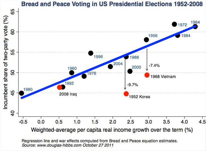
The underlying logic driving the Hibbs’ model is the idea that I have addressed in previous posts: that presidential elections are largely retrospective referendums on the performance of the party in power. Note that typically this referendum centers on the incumbent party’s handling of the economy; as this chart shows, Hibbs’ disposable income variable does a good job predicting election outcomes since 1952 all by itself.
 You can see, however, that the economic variable didn’t do very well in 1952 or 1968; in both cases the incumbent party’s candidate did much worse than economic conditions seemingly warranted. The reason why, Hibbs’ argues, is because voters were blaming the incumbent party’s candidate for unpopular wars in Korea and Vietnam. Hence the addition of the fatalities variable in his model. Note that this variable will come into play, according to Hibbs, in 2012, since Obama chose to escalate the U.S. military presence in Afghanistan. But, as we’ll see below, it won’t have nearly the impact on Obama’s vote share that the slow growth in disposable income will have.
Note that Hibbs shows particular disdain for forecast models that include what he views as ad hoc variables designed to better fit the prediction to actual election outcomes, but which add nothing theoretically. Thus, in contrast to the Abramowitz model that I’ve discussed here and at the Economist DIA site, he has no use for presidential approval variables. Although knowing how popular a president is may improve the forecast’s accuracy, it doesn’t tell us why the President has this approval rating. Presumably it has something to do with the state of the economy – but Hibbs already accounts for that. (Indeed, he finds that his “bread” and “peace” variables account for almost half the variation in presidential approval ratings). So in his view approval ratings aren’t very helpful in understanding what causes a particular election outcome.
For somewhat different reasons he dismisses the inclusion of time-related variables, including that used by Abramowitz, that punish or reward a president depending on how long his party has held the presidency. As Hibbs writes, “I regard the rationalizations of the time-coded variables …as fanciful and ad-hoc.” He shows that when these time variables are removed from some of the more well-known forecast models, their predictive capacity drops substantially.
I’ve gone through Hibbs model in some detail to remind you of two points I made in my exchanges with Nate Silver regarding the difference between political science forecast models and what Silver does. First, Hibbs’ entire forecast model is open to scrutiny by others, so that when it goes wrong, we can see why. And that gets to the purpose of this forecasting enterprise: political scientists want to do more than simply predict the outcome of an election. Doing that is quite easy: just aggregate all the most recent state level polls on the day before the election. You will hit the final Electoral College vote tally almost squarely on the head. But that doesn’t tell you why someone won the election – for that you need a theoretical explanation that you can put to the test. Hibbs’ theory says voters in 2012 will vote largely on the basis of their evaluation of Obama’s handling of the economy and, to a lesser extent, the fatalities resulting from his decision to escalate the U.S. military presence in Afghanistan.
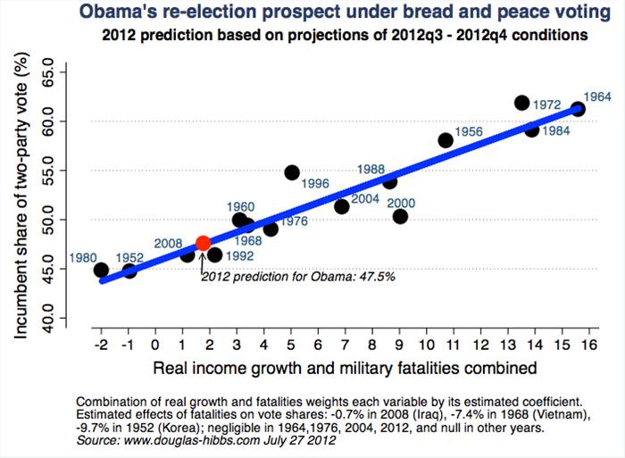
So this brings us to Hibbs’ prediction for 2012. Looking only at disposable income alone, he argues the situation does not look good for Obama; the weighted average quarterly growth rate since Obama took office is only .1%, far below the post-World War II average of 1.8%. His model suggests that the U.S. has to experience at least 1.2% growth for a president to win 50% of the two-party vote. Barring spectacular growth in the next two quarters, then, Obama is going to fall short of rate needed to win a 50% share of the vote. When you include the Afghanistan-related casualties – actual and projected – and assuming a growth rate in disposable income of between 1 and 2% in the last two quarters of 2012, Hibbs’ projects that Obama will likely lose the election, garnering only about 47.5% of the two-party vote.
 As he readily acknowledges, his forecast is something of an outlier compared to the predictions of several other political science models, including Abramowitz’s, that forecast a narrow Obama victory. Nonetheless, he is sticking by his model, albeit with the understanding that some unforeseen event or idiosyncratic factors related to this election could through his projection out of whack.
What might those be? If you look at the graph above, you’ll see that his forecast model didn’t do a very good job in either 1996, where it underestimated Clinton’s vote share, or in 2000, when it overestimated Gore’s vote share. He thinks Clinton’s legendary “charm” and Gore’s rather wooden campaign style may have thrown his projections off. Of course, as I’ve noted in earlier posts, almost none of the forecast models did well in 2000, a fact that some analysts attribute to Gore’s poor campaign strategy. Looking toward 2012, Hibbs acknowledges the possibility that idiosyncratic factors associated with election-year issues and candidate characteristics could come into play. Among the former are controversies regarding gay marriage and immigration policy and the recent Court ruling upholding the Affordable Care Act. Of the latter, Romney’s Mormon faith could turn some voters away. Interestingly, Hibbs does not view Obama’s race as one of them, declaring that because of Obama’s 2008 victory: “Race will never again figure significantly in presidential politics, and that will be Obama’s greatest positive legacy to Democracy in America.”
Note that the Hibbs model is not without its critics. As Harry Enten tweeted, one might take Hibbs to task for the rather ad hoc nature of his estimate of the impact of fatalities on vote share, which varies by wars. Moreover, Hibbs gives presidents a “one-term grace” period for wars inherited from a previous administration of the opposing party. Some might argue that this is no less ad hoc than the inclusion of a time variable that rewards the incumbent party for holding office for one term, but penalizes that party after three presidential terms. The important point, of course, is that we can make these criticisms because Hibbs shows us his model, warts and all.
And this brings me to a more general point. In 2008, as I noted in my Economist post, political scientists seeking to predict the outcome of the presidential race had it rather easy, since the contest was not that close. Every forecast model, save one, predicted Obama’s victory. However, it may very well be the case that in 2012, the forecast models will be equally accurate in terms of projecting the likely vote share, but that a number of them won’t get the winner right. That’s because the forecasters usually construct a confidence interval along with their forecast – that is, they are really estimating the probability that a candidate’s share of the major party vote will fall within an upper and lower value. So, for example, if a forecast model projects Obama to win just over 50% of the vote, but with a 95% confidence interval ranging from 49.1 to 51.1, and Obama ends up losing the election with 49.3% of the vote, that is still a pretty damn good projection by political science standards. That is, the model worked as well as any forecast model can hope to work, even if it didn’t predict the winner. This point, of course, will be lost in the post-mortem of the “incorrect” forecast models by critics, but it’s worth stating now because by all measures to date this election remains one of the closest in recent memory – one that may be too close to call given the uncertainty associated with most forecast models.
And this is a reminder, once again, that for political scientists, predicting the election winner is a means to an end – it’s not the end itself.
UPDATE: 12:50. Since I’ve already gotten several emails about this – yes, I think there are potential flaws in Hibbs’ model. To begin, he has decided that Obama will pay a penalty for the casualties resulting from the Afghanistan “surge” he initiated. To Hibbs, this evidently counts as an unprovoked war. But one might easily argue that he inherited the war from Bush, and that he established a deadline to withdraw troops after the surge – and was it really an unprovoked war in any case? Add to that the credit he will receive for orchestrating Bin Laden’s death and maybe the negative impact of the war will actually be a positive? On the other hand, Hibbs’ final estimate doesn’t put much weight on the war variable – it costs Obama maybe .25% of the popular vote share. His estimate is almost entirely a function of the sluggish economy. And Hibbs’ model does have a good track record.
*Hat tip to Mo Fiorina for alerting me that the latest Hibbs’ forecast was up.
