Monthly Archives: August 2012

The State of The Race: It Was The Best Of Times. It Was The Worst Of Times.

Today saw two separate and seemingly contrasting assessments of the state of the 2012 presidential election.  First, CNN released its latest presidential poll, and it showed Barack Obama leading Mitt Romney among a sample of registered voters by 52%-47%.  Later, Fox News released its own survey showing Obama up among registered voters by 9%, 49%-40%, over Romney.  At the same time as these generally favorable polls for Obama were released, political scientist James Campbell, in this guest column at Larry Sabato’s Crystal Ball, weighed in with his own assessment of the election that painted a distinctly different picture.   Campbell analyzed two sets of numbers: second quarter GDP numbers in the election year, and GDP numbers for the last 10 fiscal quarters prior to the election in presidencies starting back to 1956 through the Obama administration, and correlated them with elections results.  He found that by both measures the economy under Obama ranks near the bottom of the pack – a finding that, if history holds, does not bode well for Obama’s reelection chances.  As Campbell writes, “If the election becomes largely a referendum on President Obama’s economic record, it is hard to see how he can win. As I have been setting it out in this essay, the record really speaks for itself. It is dismal, and this is without noting the 42 consecutive months and counting of an unemployment rate over 8%.”

How do we reconcile polls results such as those contained in the CNN and Fox surveys that show Obama ahead with the much more pessimistic forecasts by political scientists, such as Doug Hibbs, Campbell and even Alan Abramowitz, based on economic fundamentals?  Bert Johnson and I touched on this topic in our latest professor pundits’ video, but I want to elaborate some of our comments here. In a scholarly article written  in 1993, Gary King and Andrew Gelman examined why trial heat polls like CNN’s and Fox’s can be so volatile in the months preceding a campaign despite political scientists’ claim that election results are largely dictated by fundamental factors that do not change appreciably during the campaign season.   The answer, they suggest, is that many voters who are surveyed several months before an election often really haven’t given much thought to who they will vote for, even though they respond to the question sincerely.   That is, these survey respondents over estimate their own certitude regarding for whom they are likely to vote.  But their answers this far out are often driven by short-term events, such as media coverage of a candidate’s “gaffe”, or more general perceptions regarding who is “ahead” in the race.  These short-term factors, however, are not the ones that ultimately drive the decision for most individual voters.  Instead, that decision will be rooted in the fundamentals, such as economic growth as measured by GDP, as interpreted through voters’ own partisan and ideological lens.

Although their research is dated, I don’t think King and Gelman’s conclusion are any less applicable today, which is why I caution against paying much attention to trial heat polls such as CNN’s and Fox’s at this stage of the campaign. This is even more so for state- level trial heat polls, which is why I am skeptical of efforts to predict the Electoral College vote this far out, particularly since many pollsters’ likely voter screens at the state level aren’t particularly accurate as yet.   More generally, I don’t believe that the relative electoral fortunes of Obama and Romney are fluctuating as much as many voting models based on polling data suggest.

Now, as I have said many times before, when we get closer to the election these polls will become increasingly accurate and they should (fingers crossed!) converge with what the forecast models based on the fundamentals tell us should happen.   Indeed, by the final weeks of the campaign, the polls will be much more precise than our fundamental-based forecast models.   As of now, however, the fundamentals cast a gloomier outlook on the election for Obama than do today’s trial heat polls.  How gloomy? Here, according to Campbell, is where Obama’s 2nd quarter GDP numbers rank among presidents dating back to 1952:

As you can see, only Carter had a worse election year second quarter.  The story is not much better if we look at the average GDP growth for the last 10 quarters; here the GDP figures for Obama are better only than George H.W. Bush’s and the Nixon-Ford quarters.

Note that Campbell doesn’t actual present a forecast in this article.  In past years, however, he has presented a forecast model in early September based on GDP 2nd quarter growth and Gallup Poll trial heat polls from Labor Day, and I expect he will do so again in a matter of weeks. In previous elections this model has done quite well predicting the winner’s share of the two-party vote. Like all forecast models, however, it is not foolproof; in 2008 Campbell was the only political scientist to my knowledge who forecast a McCain victory (with 52.7% of the two-party popular vote).  Ironically, Campbell blames his failure to forecast Obama’s victory on one of those “black swan” events that political scientists always say can throw a forecast off, but which never seem to appear.  In 2008, however, if Campbell is to be believed, it did appear in the form of the Wall St. meltdown. As Campbell wrote in his election post-mortem (gated): “Unlike any election in modern history, the 2008 campaign had been derailed by an entirely unanticipated and unpredicted external event.”    But, given this unprecedented fiscal meltdown, why did the other forecast models successfully predict Obama’s victory and come much closer to estimating his share of the two-party vote?  Campbell says, in essence, that they were lucky:  “Under the circumstances, I think that whether a forecast was close to or distant from the vote this year is largely a matter of good or bad luck.  Nothing in any of the models would have either directly or indirectly anticipated the effects of the timing of the Wall St. meltdown.  Nothing.”

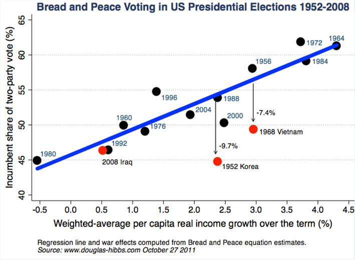
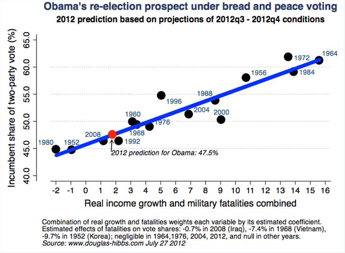
Not all forecasters would agree.  As I noted in an this earlier post discussing Doug Hibbs’ forecast model, Hibbs has no use for models like Campbell’s that incorporate trial heat polls or presidential approval ratings because they are essentially adding “noise” the forecast, since both approval and trial heat results are themselves predicated, at least in part, on the economic fundamentals.

So where does that leave the race?  In my view, the fundamentals that have generally proved reliable in the past suggest that come November, this race will be much closer than the margin suggested by today’s CNN and Fox polls.  Although you will undoubtedly hear pundits proclaiming in the wake of these latest polls that we are seeing a potential turning point in the race, with Obama beginning to stretch his lead, the King and Gelman study reminds us that this type of polling volatility is par for the course and likely does not provide a very reliable preview of November’s outcome.

The 2012 Presidential Election Is Most Like This Previous Election

One of the recurring exercises in any presidential election year is the effort by pundits to find the most appropriate historical analogue among previous presidential elections.  What is deemed “appropriate”, however, is usually determined by whether the historical antecedent favors your preferred candidate.  This election cycle has been no exception.  Democrats see strong parallels between the current race and the 2004 contest between John Kerry and George W. Bush.  Although Kerry actually led in some early polls, the election remained quite close until Bush, the first-term incumbent running for reelection, pulled it out with slightly more than 51% of the two-party popular vote. Not surprisingly, Romney supporters don’t believe 2004 has much to say about this election. Instead, they point to 1980, when Ronald Reagan trailed Jimmy Carter in the Gallup Poll for much of the post-Labor Day period only to surge ahead in the closing week, as the most fitting historical parallel.

In this vein, Greg Sargent, writing in yesterday’s Plum Line column for the Washington Post, took issue with the 1980 comparison for several reasons.  The first has to do with the difference in candidate qualities; Sargent writes:   “Reason one: Obama is a better and more likable politician than Jimmy Carter was, and Romney has not proven himself to be Ronald Reagan.”  As evidence, Sargent quotes long-time GOP strategist Ed Rollins who notes that Romney is no Reagan: “There’s no question that on his best day, he’s not a Ronald Reagan…. Traditionally incumbents don’t do as well in debates as challengers for the simple reason that challengers have to stand on the stage and look like an equal. Romney can do that, but Obama is good. He’s likeable. Carter was never likeable.”

If asked, I think many pundits would agree with Rollins’ characterization of Carter; he was the moralizing, preachy politician who – with a smugness bordering on arrogance – castigated Americans for their “crisis of confidence”.   It was small wonder that he was viewed as so much less likable when compared to Reagan – the eternal optimist who spouted homilies about America as the shining “city on a hill”.  Not surprisingly, Reagan pulled ahead after their one and only debate in late October, largely because voters had a stronger personal affinity with  Reagan.  The lesson?  Reagan’s sunny optimism trumped Carter’s dour moralizing.

Alas, Rollins has the story completely backward, as Mo Fiorina reminded us earlier in this this New York Times editorial which I’ve discussed before.    Rather than being disliked, on a personal level Carter was held in far higher regard than Reagan in the eyes of most voters – indeed, despite his low job approval, Carter had the highest-rated personal qualities of any Democratic candidate in the period from 1952-2000, and Reagan had the lowest of any Republican presidential candidate. As Fiorina summarizes: “The Ronald Reagan of October 1980 was not the Reagan of “morning again in America” in 1984, let alone the beloved focus of national mourning in 2004. Many Americans saw the 1980 Reagan as uninformed, reckless, and given to gaffes and wild claims. But despite their misgivings about Reagan, and their view that Carter was a peach of a guy personally, voters opted against four more years of Carter.”

As is often the case, the prevailing view of Carter as unlikeable likely reflects a post-hoc rationalization for why he lost the election, as well as eight years of a largely successful Reagan presidency.  But that’s not how the two candidates were viewed in the run-up to the 1980 election – something Rollins evidently forgets.

But perhaps there’s a second good reason why this year isn’t like 1980? Sargent, again citing Rollins, argues: “Reason two: The electorate is far more polarized now. Rollins notes that a last-minute shift was enabled by the larger role Dem swing voters played at the time. ‘There was a big swing element in the Democratic Party — blue collar Democrats,’ Rollins noted. ‘It’s smaller now.’

Again, I think this analysis is at least in part wrong; as I’ve argued in many previous posts (see here, for example) there’s not much evidence that the electorate is more polarized now than in previous elections.  What has changed is that the choices have become more polarizing.  This may make it less likely that voters of one party will consider voting for the opposing party’s candidate.  But it does not mean that there are not enough undecided voters left to preclude a small shift toward Romney in the closing weeks of this race – and in a tight race, a small shift will be enough.

Is that likely to happen?  I don’t know.  But if it does, it almost surely will have little to do with which candidate is more likeable and instead will turn on more deep-seated voter concerns regarding which candidate is better able to resurrect a moribund economy.  In this respect, 2012 has a lot in common with 1980 – and with 2004 – and with most of the presidential elections in the post-World War II era.

3:45 p.m. I’ve added a link to the Gallup data showing Carter leading Reagan during most of the post-Labor Day general election campaign until Reagan surges near the end.  Note that the race was quite tight for most of this period, according to Gallup.

An Electoral Landslide For Obama?

Michael Tomasky wrote a provocative online piece yesterday in the Daily Beast in which he speculated that Obama may, in fact, be on the verge of winning an electoral landslide.  Tomasky wrote, “The secret is the electoral college, and the fact is that the more you look at it, the more you come to conclude that Mitt Romney has to draw an inside straight like you’ve never ever seen in a movie to win this thing…. the paths to 270 are few.”   In looking at the key battleground states, Tomasky concludes that, given current polling, it is very unlikely that Romney will win enough of them to secure an Electoral College majority.  “In other words, Obama can lose the big Eastern four—Ohio, Virginia, North Carolina, and Florida: all of ’em!—and still be reelected. And barring some huge cataclysm, he’s not losing all four of those states. If he wins even one—say Virginia, the smallest of the four—then Romney has to win Colorado, Iowa, and New Hampshire; all possible, certainly, but all states where he has been behind, narrowly but consistently, for weeks or months.”

At first read, Tomasky’s logic seems persuasive.  After all, Romney might squeak out a victory in one or two of the battleground states.  But is it realistic to expect him to win the “big four”  – “all of ‘em!” – and the additional battleground states he needs to claim victory?  Consider the state of the Electoral College map right now.  Obama is likely starting from a baseline of some 179 electoral votes, compared to 131 for Romney.  If we add the “leaning” states to each candidates’ column, Obama moves to 247, while Romney is only at 191.  That leaves 100 electoral votes across eight states still in play.  Let’s say that Tomasky is right and that Obama is not going to lose all of the eastern  “Big Four”.   Since Obama is up almost 5 points in state polling in Ohio,  let’s assume Obama will win that, putting him at 265 electoral votes, only five short of the majority he needs to win. That would mean that of the remaining  seven battleground states, Romney would need to win six: a seemingly daunting task.

The problem with this type of analysis is that it implicitly treats the outcome in each state as an independent event.   But they are not independent;  the factors that influence how well  Romney does in Florida – say, voters’ perception of the national economy – will also affect his performance in the other battleground states.  So if in the last weeks the undecideds break his way in one battleground state, they are likely to do so in all of them.  And it won’t take a “cataclysm” to push Romney over the top – he’s within 3% in six of the eight battleground states based on the RealClearPolitics aggregate polling right now. This is not to say that local factors don’t matter at all – they do.  And in a close election, they could be decisive.  But national factors also come into play here, and that means it is not as improbable as you might think from reading Tomasky’s analysis that one candidate might end up sweeping almost all the closely contested races.   Put another way,  if Romney wins the national popular vote, it is likely he’s going to win enough of the battleground states to claim victory in the Electoral College as well.  The same holds, however, for Obama: if most of the remaining undecideds decide he deserves  more time to right the economy, he might very well coast to an Electoral College victory.  But he will likely do so primarily on the basis of a national tide – not local currents.

Obama Up By Ten? “Pew!” Say Republicans!

Romney supporters were up in arms regarding a Pew poll released two days ago of 1,956 registered voters that showed Obama leading Romney by 10%, 51%-41%. Much of the controversy centered on Pew’s sample of registered voters, which included 459 self-identified Republicans compared to 813 Democrats, with the remaining 684 declaring as independents. Critics argued this partisan distribution was heavily and unfairly skewed toward Democratic respondents.   They pointed out that the partisan difference in 2008 – a strong Democratic year – was only 7- in favor of Democrats according to the CNN exit polls, and that two years ago the parties were evenly divided in the midterm elections.  But the Pew poll suggests that partisan advantage has almost doubled.

How can Obama be up by 10%, particularly when the forecast models I’ve discussed in previous posts based on the fundamentals suggest that in contrast to 2008, this race is practically a dead heat?  To understand the seeming discrepancy, you should keep four key points in mind. First, remember that Pew doesn’t simply report the raw sample results; they do adjust the sample to bring it in line with broader demographic variables such as race, ethnicity, and even cell phone use.  So, Obama’s final margin is based on a weighted sample of 38% Democrats, 25% Republicans, and 33% independents – not the 41% Democrat subsample that some sources reported yesterday.

However, Pew does not adjust based on partisan self-identification – that is, they don’t try to “match” the sample to some national distribution of Democrats and Republicans. Critics who think they should do so are mistaking the nature of partisan self-identification in these polls.  Often, they confuse self-professed party identification with party registration data. Party identification is an attitude – not a demographic figure akin to one’s religion, or race, or ethnicity.  As such, although partisan identification is generally stable on the whole, it can change, and often does in response to how survey respondents are reacting to the current race and candidates.  As evidence, consider this chart from Pew that shows the changes in party self-identification dating back one year.

You can see that the number of self-professed Democrats and Republicans has varied by as much as 8% during this period.  Yes, yesterday’s sample contained a relatively high number of Democrats, but the average partisan Democratic lean across this period is about 7%.  Keeping in mind that there is always some random variation in probability sampling, a 10% Democrat skew is not unexpected in a Pew poll, given changes in past partisan distributions among registered voters.

Third, as I noted many times before, polling organizations like Pew all have their own house formulas for choosing a survey sample and deciding how to weight survey results.  Pew’s methodology has consistently produced results that show Obama leading Romney in head-to-head matchups.   Other polling firms, such as Gallup, show this to be a much tighter race.  It is for this reason that I have long cautioned against relying on any single poll to gauge the state of the race.  But neither should you discount any poll, such as Pew, just because you don’t like their results.  Instead, I prefer to rely on the aggregate tracking polls, such as those at RealClearPolitics or Pollster.com.  Although they also have their own methodological bias based on how quickly they adjust trend lines to the latest polls, and the degree of “smoothing” they use to handle polling outliers, I think they give a better indication of the actual state of the race than does any single polling outfit.

What do they show?  As of yesterday, the RealClearPolitics “poll of the polls” has Obama up over Romney by 2.7%, 47.3%-44.6%.  The Pollster.com aggregate poll, meanwhile, shows the race dead even with both candidates pulling in 46.1% of the vote.  For what it’s worth, the TPM poll tracker has Romney up by .6%, 46.3%-45.7%, but since this is a left-leaning partisan site I don’t normally look at the polling data there.

The aggregate polls, then, indicate that this is a very close race – one that is too close to call.  That is consistent with at least some of the political science forecast models I’ve discussed in previous posts.  Note also that at this point most polling firms are still sampling registered and not likely voters for the simple reason that their likely voter screens don’t achieve a high level of accuracy until we get closer to Election Day.  Historically, for reasons dealing with education, income and other factors related to voting, the pool of likely voters skews a bit more Republican than does the one based on registered voters.

A final point. Several of you have emailed arguing that based on Electoral College forecast models, Obama has a much bigger lead than is indicated by the popular vote.  At this point, however, I’m not ready to pay much attention to state-level polling and Electoral College projections, in part because there’s not always enough state level polls on which to gauge the likely outcome. But even at the national level, polls are still not nearly as predictive as they will be in another month, as this graph based on research by Chris Wezlien and Robert Erickson indicates:

Moreover, history says that it is highly unlikely that the winner of the popular vote is not going to take the Electoral College as well. Yes, there are exceptions – and this year might be one of those. Of course, at some point shortly before Election Day, these state-level polls will become numerous and accurate enough to project state winners and to calculate an Electoral College result.  Until then, however, I don’t see much point paying any attention to state-level projections. The aggregate polls tell us pretty much what we can hope to know at this stage of the race – and they suggest a very close contest.

No Bread, No Victory: Why Obama Might Lose in 2012

Another day, another political science forecast.  This one, Professor Doug Hibbs’ Bread and Peace model, is one of the more parsimonious forecast efforts around.  He essentially uses two variables – a weighted average of the per capita disposable personal income growth rate across the President’s term and U.S. military fatalities in unprovoked wars – to estimate the incumbent party’s share of the major party vote.   Of the two variables, the weighted average of quarterly income growth (his personal income coefficient includes the election term growth rates dating back through the first quarter of the president’s electoral term, with most recent income growth rate carrying almost 4 times the weight as the earliest) as the single best indicator of voters’ perception of the state of the economy.  But Hibbs argues as well that a party initiating an unprovoked war will also suffer electorally, with the size of the electoral penalty increasing in proportion to the cumulative number of U.S. military casualties per capita.

The underlying logic driving the Hibbs’ model is the idea that I have addressed in previous posts: that presidential elections are largely retrospective referendums on the performance of the party in power.  Note that typically this referendum centers on the incumbent party’s handling of the economy; as this chart shows, Hibbs’ disposable income variable does a good job predicting election outcomes since 1952 all by itself.

You can see, however, that the economic variable didn’t do very well in 1952 or 1968; in both cases the incumbent  party’s candidate did  much worse than economic conditions seemingly warranted.  The reason why, Hibbs’ argues, is because voters were blaming the incumbent party’s candidate for unpopular wars in Korea and Vietnam. Hence the addition of the fatalities variable in his model.  Note that this variable will come into play, according to Hibbs, in 2012, since Obama chose to escalate the U.S. military presence in Afghanistan.  But, as we’ll see below, it won’t have nearly the impact on Obama’s vote share that the slow growth in disposable income will have.

Note that Hibbs shows particular disdain for forecast models that include what he views as ad hoc variables designed to better fit the prediction to actual election outcomes, but which add nothing theoretically.  Thus, in contrast to the Abramowitz model that I’ve discussed here and at the Economist DIA site, he has no use for presidential approval variables.  Although knowing how popular a president is may improve the forecast’s accuracy, it doesn’t tell us why the President has this approval rating. Presumably it has something to do with the state of the economy – but Hibbs already accounts for that.  (Indeed, he finds that his “bread” and “peace” variables account for almost half the variation in presidential approval ratings).  So in his view approval ratings aren’t very helpful in understanding what causes a particular election outcome.

For somewhat different reasons he dismisses the inclusion of time-related variables, including that used by Abramowitz,  that punish or reward a president depending on how long his party has held the presidency.  As Hibbs writes, “I regard the rationalizations of the time-coded variables …as fanciful and ad-hoc.”  He shows that when these time variables are removed from some of the more well-known forecast models, their predictive capacity drops substantially.

I’ve gone through Hibbs model in some detail to remind you of two points I made in my exchanges with Nate Silver regarding the difference between political science forecast models and what Silver does.  First, Hibbs’ entire forecast model is open to scrutiny by others, so that when it goes wrong, we can see why.  And that gets to the purpose of this forecasting enterprise:  political scientists want to do more than simply predict the outcome of an election.  Doing that is quite easy: just aggregate all the most recent state level polls on the day before the election. You will hit the final Electoral College vote tally almost squarely on the head.  But that doesn’t tell you why someone won the election – for that you need a theoretical explanation that you can put to the test.  Hibbs’ theory says voters in 2012 will vote largely on the basis of their evaluation of Obama’s handling of the economy and, to a lesser extent, the fatalities resulting from his decision to escalate the U.S. military presence in Afghanistan.

So this brings us to Hibbs’ prediction for 2012.  Looking only at disposable income alone, he argues the situation does not look good for Obama; the weighted average quarterly growth rate since Obama took office is only .1%, far below the post-World War II average of 1.8%.  His model suggests that the U.S. has to experience at least 1.2% growth for a president to win 50% of the two-party vote. Barring spectacular growth in the next two quarters, then, Obama is going to fall short of rate needed to win a 50% share of the vote. When you include the  Afghanistan-related casualties – actual and projected – and assuming a growth rate in disposable income of between 1 and 2% in the last two quarters of 2012, Hibbs’ projects that Obama will likely lose the election, garnering only about 47.5% of the two-party vote.

As he readily acknowledges, his forecast is something of an outlier compared to the predictions of several other political science models, including Abramowitz’s, that forecast a narrow Obama victory. Nonetheless, he is sticking by his model, albeit with the understanding that some unforeseen event or idiosyncratic factors related to this election could through his projection out of  whack.

What might those be? If  you look  at the graph above, you’ll see that his forecast model didn’t do a very good job in either 1996, where it underestimated Clinton’s vote share, or in 2000, when it overestimated Gore’s vote share. He thinks Clinton’s legendary “charm” and Gore’s rather wooden campaign style may have thrown his projections off. Of course, as I’ve noted in earlier posts, almost none of the forecast models did well in 2000, a fact that some analysts attribute to Gore’s poor campaign strategy.  Looking toward 2012, Hibbs acknowledges the possibility that idiosyncratic factors associated with election-year issues and candidate characteristics could come into play.  Among the former are controversies regarding gay marriage and immigration policy and the recent Court ruling upholding the Affordable Care Act.  Of the latter, Romney’s Mormon faith could turn some voters away.  Interestingly, Hibbs does not view Obama’s race as one of them, declaring that because of Obama’s 2008 victory:  “Race will never again figure significantly in presidential politics, and that will be Obama’s greatest positive legacy to Democracy in America.”

Note that the Hibbs model is not without its critics. As Harry Enten tweeted, one might take Hibbs to task for the rather ad hoc nature of his estimate of the impact of fatalities on vote share, which varies by wars.  Moreover, Hibbs gives presidents a “one-term grace” period for wars inherited from a previous administration of the opposing party.   Some might argue that this is no less ad hoc than the inclusion of a time variable that rewards the incumbent party for holding office for one term, but penalizes that party after three presidential terms.  The important point, of course, is that we can make these criticisms because Hibbs shows us his model, warts and all.

And this brings me to a more general point.  In 2008, as I noted in my Economist post, political  scientists seeking to predict the outcome of the  presidential race had it rather easy, since the contest was not that close.  Every forecast model, save one, predicted Obama’s victory. However, it may very well be the case that in 2012, the forecast models will be equally accurate in terms of projecting the likely vote share, but that a number of them won’t get the winner right. That’s because the forecasters usually construct a confidence interval along with their forecast – that is, they are really estimating the probability that a candidate’s share of the major party vote will fall within an upper and lower value. So, for example, if a forecast model projects Obama to win just over 50% of the vote, but with a 95% confidence interval ranging from 49.1 to 51.1, and Obama ends up losing the election with 49.3% of the vote,  that is still a pretty damn good projection by political science standards.  That is, the model worked as well as any forecast model can hope to work, even if it didn’t predict the winner. This point, of course, will be lost in the post-mortem of the “incorrect” forecast models by critics, but it’s worth stating now because by all measures to date this election remains one of the closest in recent memory – one that may be too close to call given the uncertainty associated with most forecast models.

And this is a reminder, once again, that for political scientists,  predicting the election winner is a means to an end – it’s not the end itself.

UPDATE: 12:50.  Since I’ve already gotten several emails about this – yes, I think there are potential flaws in Hibbs’ model.  To begin, he has decided that Obama will pay a penalty for the casualties resulting from the Afghanistan “surge” he initiated. To Hibbs,  this evidently counts as an unprovoked war.  But one might easily argue that he inherited the war from Bush, and that he established a deadline to withdraw troops after the surge – and was it really an unprovoked war in any case?  Add to that the credit he will receive for orchestrating Bin Laden’s death and maybe the negative impact of the war will actually be a positive?  On the other hand, Hibbs’ final estimate doesn’t put  much weight on the  war variable – it costs Obama maybe .25% of the popular vote share.  His estimate is almost entirely a function of the sluggish economy.  And Hibbs’ model does have a good track  record.

*Hat tip to Mo Fiorina for alerting me that the latest Hibbs’ forecast was up.