
adapted by M. J. Simpson and R. Sandwick from a lab originally written by by K. Jewett and S. Sontum

Learning goals: analyze experimental data, formulate a logical conclusion, explain likely sources of experimental error
Introduction
A basic understanding of statistics is required in most scientific disciplines in order to analyze experimental data. For example, statistical analysis tells a pharmaceutical company whether or not a new drug is effective. One of the most common statistical tests is Student’s t-test, which helps to determine whether two populations are significantly different. The critical value that comes out of a t-test represents the probability that the populations are NOT significantly different. A common definition of “statistical significance” is p < 0.05, although this has been a topic of recent debate. This laboratory is designed to give you an introduction to routine techniques such as weighing and performing basic calculations and statistics.
Background
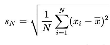
In 1795 at the age of eighteen a German mathematician Karl Friedrich Gauss devised the Gaussian curve or normal distribution (symmetrical about the average) in which the scatter of a data set is summarized by the standard deviation, or spread, of the curve. Gauss found that the best estimate of the area of uncertainty was the standard deviation, which for N measurements is given by:
The Gaussian curve has turned out to be a nearly universal description of the distribution of random data sets. Student’s grades measured by an exam follow this bell shaped curve, as well as the distribution of the weight of each grain of wheat in a field or the repeated measurements of the weight of a single wheat grain. In the bell shaped Gaussian curves depicted above, 67 % of the points fall within one standard deviation on each side of the average while 95 % of the points are with ± 2 standard deviations around the average.
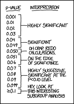
http://imgs.xkcd.com/comics/p_values.png
When two averages are two standard deviations or more apart we can say they are significantly different at a 95% confidence level, which corresponds to p = 0.05. The smaller the p value, the more confident you can be that the two averages are significantly different.
In today’s lab, you will determine whether or not there are more than one kind of U.S. minted penny based on the mass of the pennies. You will record the masses of pennies, perform statistical analysis on the raw data, and draw conclusions based on those analyses.
Procedure
Each group will pick 20 pennies out of the pool. Weigh each to four decimal places and record the mass and the year in a table. If you have never used an analytical balance before, consider reviewing this information.

Statistical Analysis
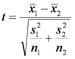
Try to group the pennies into two groups with significantly different average masses. Calculate the averages and standard deviation for the two groups. Then, calculate the p-value for the hypothesis that there are two kinds of U.S. minted pennies. This is the equation for the t-value, which you can use to look up the p-value on the t-table. Alternatively, you may use Excel or some other software to calculate the p-value, but you must understand the math in order to answer the post-lab questions. Here is an example to show you how to do the math on Google Sheets.
Note: the number of significant digits for the average depends on the standard deviation. The last significant digit of the average is the first decimal place in the standard deviation. For example, if your average is 3.025622 g and your standard deviation is 0.01845 g, then this is the correct number of significant figures for the average: 3.03 g, because the first digit of the standard deviation is in the hundredths place, so the last significant digit of the average is in the hundredths place. For the p-value, just report the range. For more information about significant figures, refer to this tutorial.
Report: Fill out the worksheet for the report. Turn in either a paper or digital copy. Optional survey.