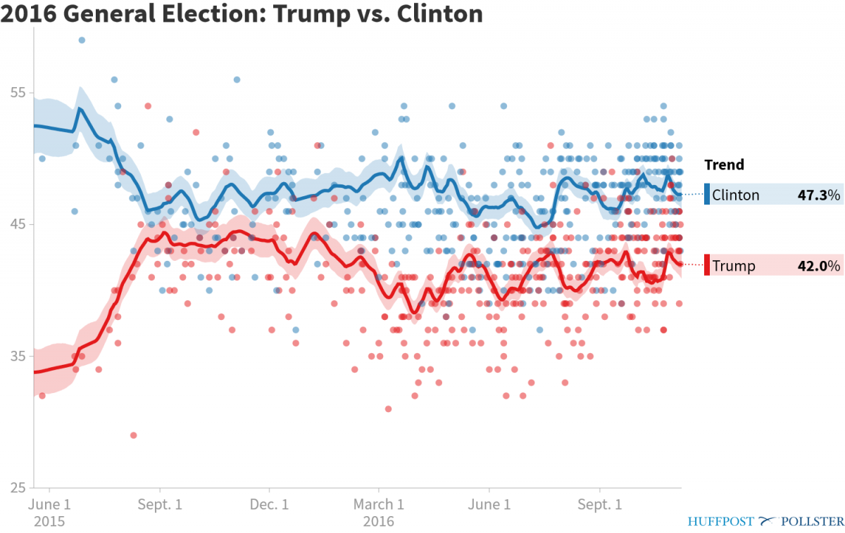
In life, they say, timing is everything. When I began doing my election-themed talks in late summer, after it was clear who the general election candidates were, Hillary Clinton consistently held a lead in the various aggregate polling results, such this one by Huffington Post, by about 5%-8%.
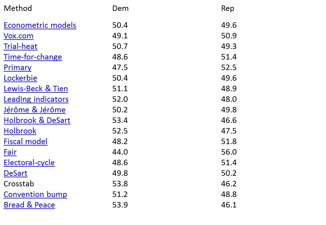
Nonetheless, I assured my audiences that there were good reasons to expect this race to tighten during the next two months. As evidence, I cited the political science forecast models which, again looked at in the aggregate, seemed to indicate that this race was going to be a dead heat. As long time readers know, these models attempt to predict the two-party presidential popular vote as a function of the “fundamentals” – that is, how well the economy is doing, whether the country is at war, and how long the incumbent party has held the White House, to name some of the most frequently utilized variables. While not perfect, and keeping in mind that they differ in the particulars, and thus in the final forecasts, these models nonetheless provide a decent template for understanding the context which both candidates then try to exploit in their favor. Simply put, when things are going well, the incumbent party candidate should try to run a clarifying campaign, to use Lyn Vavreck’s term, while the opponent will seek to focus the message on something else less favorable to the party in power. Assuming candidates make proper use of these fundamentals, the forecast models issued by Labor Day are a reliable, if not perfect, indicator of how the race will turn out. With that in mind, the key slide in my talks, which never failed to elicit a crowd reaction, was this one:
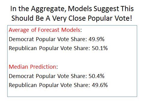
This was based on the political science forecast models available at the time – subsequent ones changed this aggregate forecast slightly at the margins, but the essential point remained: this election was too close to call, and could go either way. That, of course, was not what most of my audiences wanted to hear. As it turned out, however, the political science models – looked at in the aggregate, (which is how I typically made my prediction every four years) – were spot on in 2016. As of today, with votes still coming in, Clinton has won about 50.2% of the two-party popular vote – or almost exactly what the political science median forecast predicted.
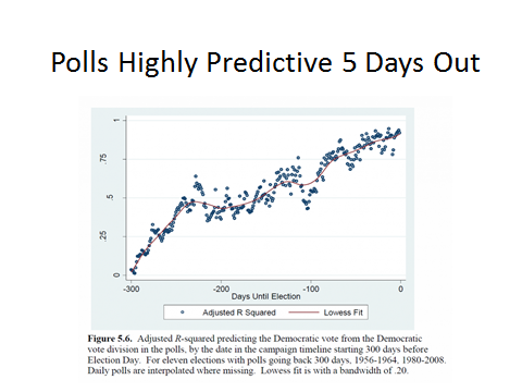
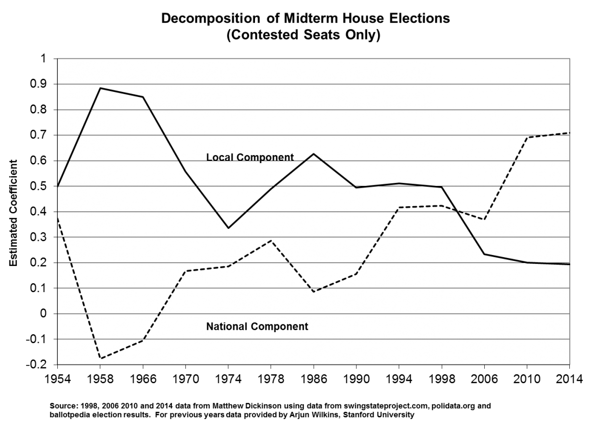
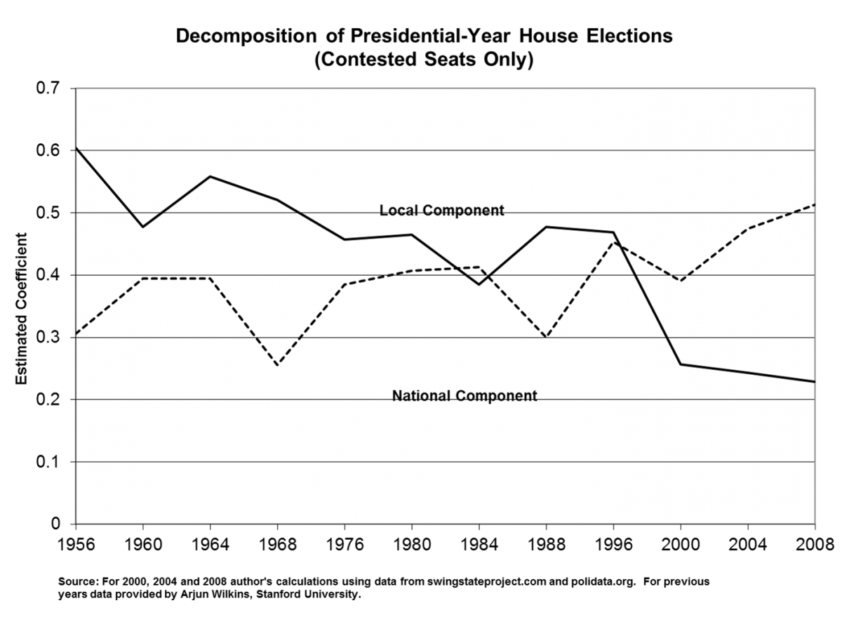
How, then, to explain those polls showing that Clinton was in the lead? Early in the campaign season, I told my audiences that, assuming Trump and Clinton ran effective campaigns – that is, that they made effective use of the fundamentals in crafting their respective messages, the polling gap between the two should close. Indeed, there is extensive evidence from previous elections, as documented by Erickson and Wlezien, that as the campaign progresses, partisans come home to roost in a way that tends to lead to a tightening in the polls. However, as the election droned on, it became increasingly clear that in my talks I had to address the 800-pound hairdo in the room: Trump was not closing the gap with Clinton nearly as quickly as I anticipated. This was surprising, because as Drew Linzer and others have demonstrated, and as the graph below shows, election polls typically get increasingly accurate as the potential voters begin tuning in and become more informed regarding which candidate comes closer to their partisan leanings. (The y-axis in the graph is a coefficient showing how much the polling aggregate predicts the final Democratic popular vote share.)
The result, as political scientists have documented in previous presidential elections, is that as the campaign heads toward the finish line, and partisans come home to roost, the polls should prove an increasingly accurate indicator of the final vote. Indeed, Drew Linzer had correctly forecast the Electoral College vote in 2012 by updating one particular forecast model (Abramowitz’s Time for a Change model) using only state-based polls. However, in 2016 his state-level poll-based forecast consistently showed a likely Clinton victory all the way up to Election Day. Indeed on Election eve, he predicted a Clinton Electoral College victory of 323-215. And he wasn’t the only one to do so – other analysts who had made accurate polls-only predictions in the past, such as Sam Wang, were also forecasting an Electoral College victory for Clinton.
So why wasn’t Trump closing the gap so that polls came closer to the political science fundamentals-only forecast? I could think of two explanations. One was that the state polls were somehow off, and were underestimating Trump’s support. In all my talks I reminded my audience that the polls-only forecast depended on the polls being right. (Not surprisingly, many audience members have forgotten that!) The second was that he was running a sub-optimal campaign, one in which his continual missteps made it more difficult for him to capitalize on the fundamentals that predicted this was a 50/50 race. In the end, I went with Trump running a suboptimal campaign. That was probably the wrong choice. But it’s worth explaining why I made it.
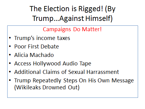
In adjudicating between the two explanations, I compared what I was seeing at Trump rallies with what prior research had shown about polling accuracy at the state level. As I’ve documented in many previous posts, Trump’s rallies were huge and enthusiastic. And in talking to his supporters, it became clear that the vast majority were not the xenophobic racists that pundits (and not a few of my colleagues) thought they were. But I worried that focusing on rallies did not give me nearly as accurate a view of the entire electorate as did the polling numbers. By the end of the campaign, I was concluding my talks by saying this was going to be a close race – one closer than the polls indicated – but unless those polls were completely wrong (and they hadn’t been in the past), Clinton was likely to win the election. I summarized the Trump-as-poor-campaigner in this slide that suggested the election WAS rigged – by Trump!:
As it turned out, however, the political science forecast models had it right, and the state-level polls did not. This is not to say that the national polls were wildly inaccurate. Indeed, as Sean Trende suggests, they were, on the whole, about as accurate as the national polls were in 2012, which on average understated Obama’s final victory margin of 3.9% by about 3.2%. It’s probably worth repeating that, as of this moment, Clinton has a popular vote lead of about 700,000 votes, or about .5% and that could grow to about 1% by the time all the votes are counted. That’s less than the RCP final four-way average which gave her about a 3.3% margin. But that’s a difference that’s actually a tad smaller than the 2012 RCP error margin. Keep in mind as well that due to the random error associated with statistical sampling, polls in the aggregate don’t usually exactly match the final vote total, even though they typically do approach that total, as I pointed out in my lectures.
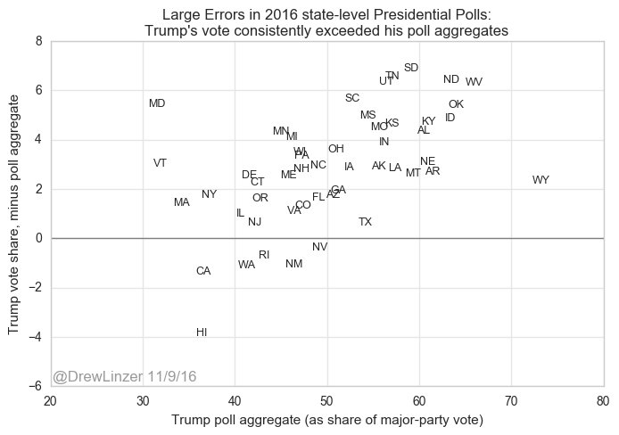
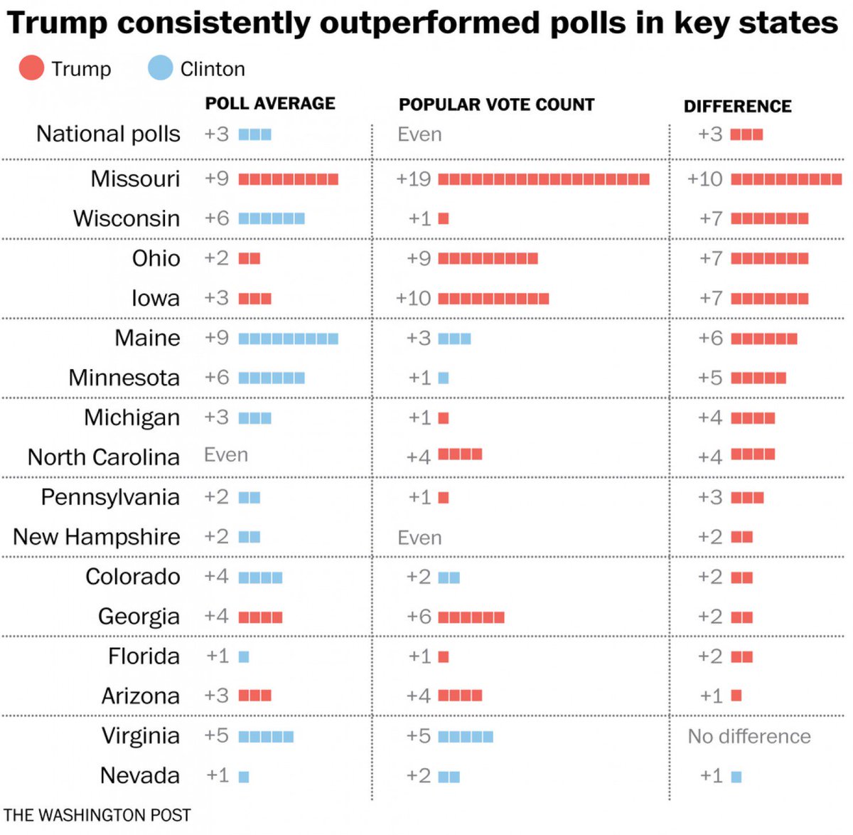
But as Linzer showed, in 2016 the state-level polls consistently underestimated Trump’s support, and that miss proved crucial in forecasting key swing states, including Wisconsin, Michigan, and Pennsylvania, which was enough to throw the Electoral College projections in the polls-only models off. Generally speaking, the polls got Clinton’s support right, but they underestimated Trump’s. This graph by Linzer reveals the extent to which the state-level polls underestimated Trump’s support.
And this Washington Post table shows how much the polls missed Trump’s support in those key states.
I will devote future blog posts to examining why the state-level polls were wrong, as I expect Linzer and others will do as well. But for now the important takeaway is that, once again, in the aggregate the political science forecast models got this right – exactly right, as it turns out (which undoubtedly will again elicit remarks about how smug we are). And they did so because this was an election governed by dynamics that were largely unchanged from previous presidential elections, as Larry Bartels points out. Bartels shows this by comparing Trump’s state-by-state performance with Romney’s 2012 results. As you can see, Trump did well in states in which Romney did well (with Utah a notable exception!) and not so well in the states in which Romney struggled.
The fact that Trump’s performance was both predicted, and that it doesn’t suggest a significant realignment in the electorate, is probably something that political pundits, whose professional existence depends on creating the impression that elections can and usually do change in reaction to every campaign event (Comey cost Clinton the election!), and that the outcome represents something new (and therefore newsworthy) may not want to hear. But it’s what the evidence suggests.
Yes, some of my colleagues are expressing mea culpas for relying too heavily on the polls in making their final projections. I understand that sentiment – by the end of the campaign season I was also telling my audiences that although the race would be close, the polls were usually pretty accurate, and that they seemed to suggest a high probability of a Clinton victory. But let’s be clear: political science got this election exactly right, even if some political scientists (like me!) weren’t smart enough to realize it. And here’s the proof, again provided courtesy of Linzer:
https://pbs.twimg.com/media/Cw3X4PbUoAA_ej2.jpg
And this is a reminder that if you want to know who is going to win the presidential election, polls are (usually!) a pretty reliable indicator, although they certainly were not as accurate at the state level this time around as they have been in previous years. But if you want to know why Trump won, the political science forecast models issued by Labor Day are a good place to start. And they suggest Trump’s victory was, in large part, fundamental.
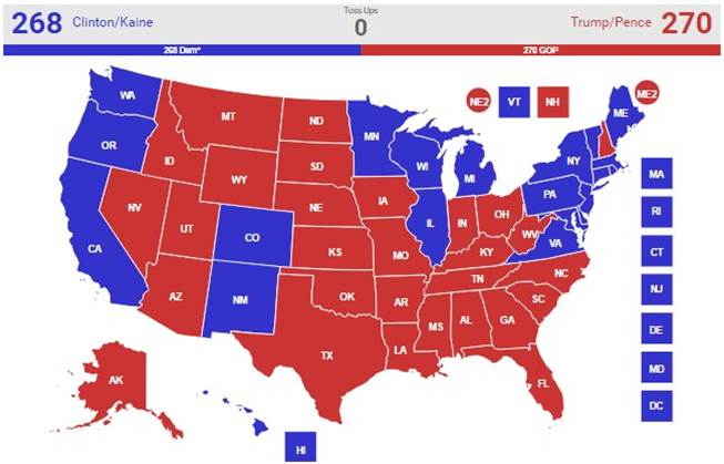 But current polls also suggest that even as Trump pulls ahead in New Hampshire, he’s still behind in Nevada and probably Florida, and it’s not clear he can hold onto North Carolina – a state Romney won in 2012. Moreover, if you play out all the possible Electoral College scenarios in this way, which is what simulations are designed to do, the odds still heavily favor Clinton. She simply has more paths to victory. Trump, in contrast, has far fewer electoral options and thus has to hope all the key states break his way – an outcome that, while not impossible, is much more improbable.