Learning goals:  follow instructions to complete a chemistry experiment, collect and analyze experimental data, explain likely sources of experimental error, work collaboratively with a lab partner.

Introduction

Rules about significant figures may seem arbitrary from a theoretical standpoint, but in the laboratory you will see that they allow you to determine the precision of your measurements and calculations. When your measurement has a limited number of digits, your subsequent calculations will also have a limited number of digits.

In this lab, you will be measuring the density of water using a variety of tools. Although your results should be similar every time, the number of significant digits you get will vary depending on the uncertainty associated with the measurement techniques.

Background

Significant digits from common measurements

1. 1. Mass – analytical balances generally give many significant digits, particularly when weighing 0.1 g or more, you get 4, 5, 6, or 7 significant digits. For example, 0.5012 g of a substance has 4 significant digits. Higher masses give you more significant digits until you reach the capacity of the balance. 319.9999g is 7 significant digits. That is the maximum mass for one of our balances.
   2. Volume
      • Volumetric flasks are extremely precise tools for measuring volume and often give you 4 or more significant digits, depending on the size of the volumetric flask. For example, a precision 1 liter volumetric flask filled exactly to the line etched on the neck contains 1.0000 L, which is 5 significant digits. The precision is usually printed on the flask for reference.
      • Micropipettes are very precise tools for measuring extremely small volumes (less than one milliliter). The number of significant digits you get from a micropipette is printed on the pipette for your reference, but it is usually about 4 significant digits.
      • Burets are very precise tools for measuring volume. Our lab is equipped with burets that measure to the nearest 0.01 mL, so a volume greater than 1 mL will have 3 significant digits, and a volume greater than 10 mL will have 4 significant digits. You always estimate one more digit than you can read from the lines and estimate to 1/5th between lines.
        

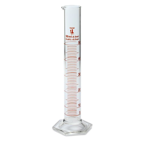
        50 mL graduated cylinder https://images-na.ssl-images-amazon.com/images/I/318fpllZXkL.jpg

      • Graduated cylinders are the most flexible tool for measuring volume. Our lab is equipped with many different graduated cylinders, and the number of significant digits they give you depends on the exact graduated cylinder you are using and the volume you are measuring. The number of decimal places you can read is printed on the glass for your reference. Typically you will get 3 significant digits from a graduated cylinder. You always estimate one more digit than you can read from the lines. You will normally estimate to the nearest 1/5th between lines.
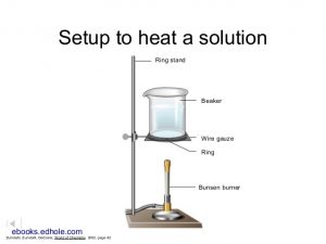
      • Repeat after me: “Erlenmeyer flasks and beakers are not designed to measure volumes,” although they can be used to get a rough estimate if the volume is not critical. For example, if you are making a hot water bath with approximately 400 mL of water (1 significant digit), then it is appropriate to use a beaker measure that volume.
   3. Temperature – our red and blue alcohol thermometers are read to the nearest 0.1 °C. This means that we can only read 3 significant digits for temperatures between 10 and 99.9 °C, and we only get 2 significant digits for temperatures between 0 and 9.9 °C. You always estimate one more digit than you can read from the lines. Mercury thermometers give more significant digits, but they have fallen out of favor due to safety concerns when they (inevitably) break.

Significant digits from common calculations

1. Adding/subtracting: Use the least number of decimal places involved in the calculation. For example, if you measure a temperature change from 25.0 °C to 28.1  °C, 28.1 – 25.0 = 3.1 °C. See how fast you can lose significant digits in the lab?
2. Multiplying/dividing: Use the least number of significant digits involved in the calculation. For example, if you dissolve 0.3829 moles of a substance in 1.0000 L of water, then the concentration is 0.3829 moles per liter. The volume had 5 significant digits, but the number of moles only had 4 significant digits, so you are left with just 4 significant digits in your answer.
3. Averaging: We have special rules for averaging multiple measurements. Ideally, if you measure the same thing 3 times, you should get exactly the same result three times, but you usually don’t. The spread of your answers affects the number of significant digits in your average; a bigger spread leads to a less precise average. The last significant digit of the average is the first decimal place in the standard deviation. For example, if your average is 3.025622 and your standard deviation is 0.01845, then this is the correct number of significant figures for the average: 3.03, because the first digit of the standard deviation is in the hundredths place, so the last significant digit of the average is in the hundredths place.

Rules for rounding

Numbers between 6 and 9 round up.

Numbers between 1 and 4 round down.

5s round up or down to an even number. For example, if your average in lab is 92.5, the 5 would round down to 92, so an A- letter grade. If your average is 89.5, the 5 would round up to 90, so an A- letter grade.

Procedure

1. Measure the density of 5 mL of water with a graduated cylinder

Use an analytical balance to measure the mass of an empty, dry 50 mL beaker or Erlenmeyer flask. Remember to zero the balance before you use it. Record the mass in Table 1.

Measure out 5 mL of DI water with a 50-mL graduated cylinder. Read the exact volume at the bottom of the meniscus and record it in Table 1. Be sure to record all significant figures. Estimate to the nearest 1/5th mL (1/5th between lines). You will estimate the last decimal place.

Transfer the contents of the graduated cylinder to the beaker or Erlenmeyer flask. Use an analytical balance to measure the mass of the beaker that now contains 5 mL of water. Remember to zero the balance before you use it. Record the mass in Table 1.

2. Measure the density of 50 mL of water with a graduated cylinder

Use an analytical balance to measure the mass of an empty, dry 50 mL beaker or Erlenmeyer flask. Remember to zero the balance before you use it. Record the mass in Table 1.

Measure out 50 mL of DI water with a 50-mL graduated cylinder. Read the exact volume at the bottom of the meniscus and record it in Table 1. Be sure to record all significant figures. Estimate to the nearest 1/5th mL (1/5th between lines). You will estimate the last decimal place.

Transfer the contents of the graduated cylinder to the beaker or Erlenmeyer flask. Use an analytical balance to measure the mass of the beaker that now contains 50 mL of water. Remember to zero the balance before you use it. Record the mass in Table 1.

3. Measure the density of water with a volumetric flask

Use an analytical balance to measure the mass of an empty, clean, dry 100 mL beaker or Erlenmeyer flask. Remember to zero the balance before you use it. Record the mass in Table 1.

Fill a 100 mL volumetric flask with DI water until the bottom of the meniscus is exactly at the etched line. You may need to use a dropper to reach the line exactly. Record the volume to the tenth place: 100.0 mL. Record that volume in Table 1.

Transfer the contents of the volumetric flask to the beaker or Erlenmeyer flask. Use an analytical balance to measure the mass of the beaker that now contains 100 mL of water. Note that not all of the balances in the lab may be able to measure this mass. Use a different balance if you get an error. Remember to zero the balance before you use it. Record the mass in Table 1.

Data analysis

Review the rules about significant figures, then calculate the mass of water, volume of water, and density of water for each method. Fill in Table 2. Note: density = mass ÷ volume.

Report

Fill out this worksheet. Turn in either a paper or digital copy. You may use this table to look up the correct density of water at a variety of temperatures.

Introduction

The magic of hot and cold packs lies in the chemical reactions inside; they undergo a dramatic temperature change after an activation step. You may have noticed in previous experiments that sometimes dissolving a salt makes a solution warm, other times it will make the solution cold. This property of salts is the basis for many commercial hot packs and cold packs. The activation step causes the salt and the liquid to mix, which either increases or decreases the temperature, depending on the salt. In this experiment, you will measure the heats of solution for several salts.

A reusable hot pack is a little different. It contains a supersaturated salt solution, and the activation step seeds the crystallization of the salt. Then heat is released when the salt crystallizes. It is reusable because you can heat up the solution in hot water or a microwave to dissolve the salt and reform the supersaturated solution. Today, you will also make a supersaturated solution and then measure the temperature change upon crystallization, similar to a reusable hot pack.

Background

The ability of a salt to release or absorb energy upon solution is quantified as the enthalpy of solution. To measure the enthalpy of solution experimentally, we can use a solution calorimeter to measure a temperature change of a known mass:

q = mass * specific heat * ΔT

where:

mass = total mass of the combined salt and water in grams;

specific heat = specific heat of the solution. we will approximate it as the specific heat of water, which is 4.18 J/g ^oC;

ΔT = the difference between the starting temperature and final temperature in ^oC.

This gives you q for the water. Since the q for the water is the opposite of the q for the salt, you will need to switch the sign of q for water to get q for the salt. If you want to compare your answer to a literature value, you have to standardize q for the salt to ΔH^o for the salt: convert J to kJ, then divide by the number of moles of salt you used, which gives you a value in kJ/mol. Note: this conversion is only valid under conditions of constant pressure.

This is a good web resource to learn more about enthalpy of solution.

http://images.flatworldknowledge.com/averillfwk/averillfwk-fig13_001.jpg

Similarly, the ability of a salt to release or absorb energy upon crystallization from a saturated solution is quantified as the heat of fusion. Experimentally, you can measure the heat of fusion by observing a temperature change when a salt is allowed to crystalize. The calculations all work essentially the same way and the final answer is a ΔH in kilojoules/mol.

Procedure

Note: do this experiment with a partner. You need two thermometers.

Part I: Prepare a supersaturated solution

1. Thoroughly wash a 125 mL Erlenmeyer flask. Rinse with DIH2O. It does not need to be dry. Weigh the flask, and record the mass on Table 2.
2. Measure out 50 grams of sodium acetate trihydrate directly into a tared 125 mL Erlenmeyer flask. Record the exact mass on Table 2.
3. Add approximately 40 mL of DI H2O.
4. In a fume hood with the sash lowered, heat the flask gently over a bunsen burner until it starts to boil and the crystals dissolve. Using the wash bottle filled with DIH2O, rinse all of the crystals down into the water, but try not to add too much water.
5. Once the crystals are dissolved, remove the flask from the heat, put a thermometer into a split rubber stopper, lower the thermometer into the solution, stopper the top, and let it cool undisturbed. Note: If it refuses to dissolve even at boiling, then add another 1 or 2 mL of DIH2O.

Part II: Measure enthalpy of solution

To measure the enthalpy of solution, quickly add approximately 5 g of the salt to approximately 50 mL of temperature stabilized water. Put the lid in place and lower the thermometer into the solution. Swirl to dissolve while monitoring the temperature for at least 2 minutes. Be sure you are not clutching the thermometer too much with your hand, or your body heat will affect the reading. Record all temperatures to the nearest 0.2 ^oC. When measuring masses and/or volumes, choose appropriate tools to ensure that the temperature change limits the significant figures in the final answer. Pour the solution down the drain. Rinse and dry the calorimeter before performing another trial. Hint: you may want to attempt a calculation after your first trial to be sure you collected all of the data needed to complete your calculations. If time allows, discuss the results of your first trial with your instructor or TA for recommendations on improving the experiment before subsequent trials.

Part III: Measure the temperature change of crystallization

1. Check the temperature of the supersaturated solution. If the temperature is above 30 ^oC, make a cold water bath and place the flask in the cold water bath for a few minutes to cool it to 30 ^oC.
2. Without touching the thermometer, measure the temperature of the supersaturated solution. Record the temperature as the “initial temperature” on Table 2 to the nearest 0.2 ^oC.
3. Obtain a small, single crystal of the sodium acetate salt. Carefully drop it into the flask.
4. Observe the temperature change as the solution crystallizes. Record the highest temperature achieved as the “final temperature” on Table 2 to the nearest 0.2 ^oC.
5. Remove the stopper and thermometer. Weigh the solution in the Erlenmeyer flask. Record the mass on Table 2.
6. Use excess water to redissolve the salt and wash it down the drain.

Report

Use this resource to find literature values of heats of dissolution.

Complete the worksheet. Turn in either a paper or digital copy.

Learning goals: work collaboratively with a lab partner, collect and analyze experimental data, formulate a logical conclusion based on experimental data

Note: Plan on dressing in old clothes for this lab. These dyes are powerful and may permanently stain your clothes if you splash or drip them on yourself.

Introduction

Color vision provides a window into everyday chemistry. For example, the leaves change color in autumn, indicating the changing chemistry in the tree: the chlorophylls are breaking down and the tree is preparing for the winter. Tree leaf pigments absorb some wavelengths of light more than others, which is what imparts the color you see. Less commonly, pigments can emit light; one example is a fluorescent highlighter marker. In this two-week lab, you will learn about the chemical basis of color for both absorptive and emissive colored chemicals.

In today’s lab, you will measure the absorption of several food dyes, then measure the absorption of a sample of an artificially colored food or beverage of your choice. By comparing the absorption of your sample to the absorption of the food dye standards, you should be able to identify the dye(s) in your sample, although probably with some uncertainty.

Background

Colored chemicals absorb and/or emit light in the visible portion of the electromagnetic spectrum, which has a wavelength of approximately 400 – 700 nm. The color of the absorbed or emitted light depends on the amount of energy the chemical absorbed or emitted. Wavelength and energy are negatively correlated.

Absorption occurs when an electron in a chemical absorbs energy from the light, temporarily promoting the electron to a higher energy orbital. Light emission can occur when an electron relaxes back to the ground state and produces light, but emission is less common than absorption because there are many of non-radiative ways for the electron to relax.

Most chemicals are colored because they absorb light and reflect only a portion of incident light. In this case, the color that a chemical absorbs is the opposite of the color that it appears. The color wheel shows you which colors are opposite of one another. The color wheel helps you to predict the color that a chemical absorbs based on the color it appears (and vice versa). For example, beta-carotene, a pigment found in many fruits and vegetables including carrots, absorbs purple and blue light (400 – 500 nm) and reflects all of the other colors, so it appears yellow/orange. It DOES NOT emit yellow/orange light.

Mixtures of colored chemicals add a layer of complexity. For example, a beverage may appear green because it contains green dye, so it would have one absorption peak in the red, or it may appear green because it contains a mixture of blue and yellow dyes, which would together have two absorption peaks, one in the orange and one in the violet. Just like in lab 2, chemists use the physical and chemical properties of substances to separate mixtures of substances. The separation of a mixture for analysis purposes is generally called “chromatography.” You may have inadvertently done chromatography if you have ever seen black ink get wet and spread into its component dyes based on the way the dyes interact with the water and the paper. Things that appear black or brown are mostly mixtures of multiple substances that together can absorb broadly across the spectrum such as two colors opposite to one another on the color wheel. In order to really be black, something would have to absorb every color of light, which is uncommon given that energy levels are quantized (give that some time to sink in).

https://www.acs.org/content/acs/en/education/resources/highschool/chemmatters/past-issues/2015-2016/october-2015/food-colorings.html

https://www.acs.org/content/acs/en/education/resources/highschool/chemmatters/past-issues/2015-2016/october-2015/food-colorings.html

Procedure

Part 1: Prepare cotton for tie dye

(Hint: If you read through these instructions before coming to lab, plan on completing this step before the pre-lab discussion to ensure the most vibrant colors possible.)

1. Use a permanent marker to write your name on the tag of your garment.
2. Soak your garment in the sodium carbonate wash for at least 30 minutes. This solution is very basic, so wear gloves when in contact with the wash.

Part 2: Measure absorption of various food dyes and a sample of your choice

Note: perform this procedure with a partner.

First, fill out Table 1 with information about your sample. Be sure to write down any food dyes that you know are present in the sample. Do not use a sample that contains dyes or natural colors other than the ones we are testing in Table 2.

1. Fill 7 cuvettes with 1 mL of each of the food dyes, one with your sample, and one with DI H2O (9 cuvettes total). The water serves as a blank. Label your cuvettes on the top. Use a volumetric pipette to measure the 1 mL volume.
2. Set the spectrophotometer to 430 nm.
3. Blank the instrument with the water.
4. Measure and record in Table 2 of your worksheet the absorbance of each of the dyes.
5. Repeat steps 2 – 4 for the other wavelengths. Be sure to blank at every wavelength. Note: if your sample ever gives an absorbance reading greater than 1, dilute the sample by 50% and repeat the sample measurements at all wavelengths. 
6. Wash and return your cuvettes after you are finished. All of these solutions can go down the drain.

Part 3: Tie and dye cotton

1. Wring out the garment to dry it as much as you can.
2. Fold and tie with waxed sinew your garment however you like.  Here are some designs you might like to try.
   
3. Working in a foil pie pan on a surface covered in newspaper, apply the dye. Use your knowledge of the color wheel to select colors that will mix well. (Hint: colors that are next to each other on the color wheel mix well, but colors across from each other make brown/black.) Be sure to saturate the fabric with dye, but don’t put so much on that the dye pools underneath the fabric. Again, wear gloves when working with dye or it will dye your skin!
4. Wrap your garment in clean newspaper and put it in a sealed plastic bag. Place it in your cabinet and leave it there for the week.
5. Clean your foil pie pan, return it, and throw away wet newspaper.

Report

Fill out this worksheet. Turn in either a paper or digital copy. Optional survey.

Amedeo Avogadro

Introduction

Atoms and molecules are incredible tiny and weigh hardly anything, so scientists usually count them in terms of moles, which is 6.022140857 x 10²³ particles. Why? For the same reason that we measure distance in terms of miles and donuts in terms of dozens: when you are counting to big numbers, it is easier to use big units. When eating donuts, it makes more sense to count in dozens than attempt to count individual donuts, and it is simpler to tell someone that you live 5 miles down the road than 26,400 feet.

Avogadro’s number is named to honor Amedeo Avogadro who pioneered some of the molecular theory that led to the discovery of Avogadro’s number. In this lab, you will estimate the number of molecules in a monolayer of stearic acid in order to calculate Avogadro’s number.

Background

To estimate Avogadro’s number, you must count the number of molecules. Most of the time, chemists simply use the mass to count molecules because molar mass relates mass and number of molecules:

mass of carbon (g) / molar mass of carbon (g/mole) = number of moles of carbon

number of moles of carbon (moles) x 6.022 x 10²³ atoms per mole (atoms/mole) = number of atoms of carbon

However, this approach assumes you know Avogadro’s number, so we have to get a little more creative.

When measuring lots of little things, it helps to have a lot of them piled up.

Remember that molecules are physical things that take up space. One molecule is a very little thing that takes up just a little space (microscopic), but if you have a lot of them all lined up, they take up enough space for you to measure (macroscopic). When the dimensions of the stearic acid molecule are known, we can effectively count stearic acid molecules by measuring a volume of stearic acid.

Stearic acid is a non-polar hydrocarbon chain that has a polar carboxylic acid end. When you add it to water, each molecule aligns with the polar end pointing towards the water and the non-polar portion pointing up, and the molecules form a monolayer on top of the water. You can picture each molecule like a tall, skinny rectangle with dimensions 1:5.44, and the monolayer can be approximated as a cylinder. By measuring the volume and surface area of the stearic acid layer, you will be able to calculate the dimensions of the individual molecules via geometry, which is all you need to calculate the volume of the individual molecule. Comparing the volume of the monolayer to the volume of an individual molecule gives you the number of molecules in the monolayer. Since the monolayer has a known mass, and stearic acid has a known molar mass, you can calculate Avogadro’s number. Step-by-step instructions for completing the calculations are on the worksheet.

Procedure

Note: this should all take place in a hood to protect you from fumes.

Calibration of a pipet

I. Wash a 10 mL beaker (or the smallest beaker you have).

1. Wash with soap and water.
2. Rinse with ~1 mL of ammonia solution three times. Put the rinsate in the ammonia waste container.
3. Rinse with DIH2O three times.
4. Rinse with ~1 mL of acetone. Put the rinsate in the acetone waste container. Wait for the beaker to dry (a minute or two).
5. Rinse the beaker with ~1/2 mL of hexane [CAUTION!] three times. Put the rinsate in the hexane waste container.

II. Wash a 10 mL graduated cylinder.

1. Wash with soap and water.
2. Rinse with ~1 mL of acetone. Wait for it to dry.

III. Calibrate the pipet

1. Put approximately 3 mL of hexane into the clean beaker.
2. Use the pipet and the hexane in the beaker to fill the graduated cylinder up to exactly 1.0 mL. Count the number of drops it takes to fill it to 1 mL. Record the number of drops. Tips to ensure consistent drop size:
   • Have one designated dropper. Preferably whoever has steadier hands.
   • Be sure to hold the pipet straight up and down.
   • Make sure no drops stick to the side of the graduated cylinder.
   • Don’t let the dropper touch the sides of the cylinder.
   • Work slowly and be patient.
3. Pour the hexane out of the graduated cylinder and into the hexane waste container. Wait for the graduated cylinder to dry. Blowing nitrogen on the glassware will help it dry faster.
4. Repeat the calibration procedure again. Record the number of drops in 1 mL.
5. Repeat again if the first two calibration measurements are not within 10% of one another (example: 20 and 22 drops would be acceptable, but 20 and 25 drops would warrant another calibration).

Make a stearic acid monolayer

I. Prepare a large watch glass

1. Measure and record the diameter of the watch glass with your ruler.
2. Wash the watch glass with soap and water.
3. Rinse with ammonia solution. Put rinsate in the ammonia waste container.
4. Rinse thoroughly with DIH2O. Wait for it to dry.
5. Once clean, be sure to avoid getting fingerprints on it. Handle wearing gloves, and hold it on the edges.
6. Place the watch glass on a 400 mL beaker, which will simply hold it steady for you. Make sure the watch glass is parallel to the bench top.

II. Form the monolayer

1. Using your wash bottle, fill the watch glass to the brim with DIH2O.
2. Pour about 3 mL of the stearic acid solution into the clean 10 mL beaker.
3. Fill the pipet with the stearic acid solution. Holding it straight up and down, add one drop of stearic acid solution to the water-filled watch glass. If the watch glass is sufficiently clean, the drop should disappear quickly.
4. Add the stearic acid solution drop wise until the last drop, which will remain a lens and not disappear. Record the number of drops you used. You will know you are close when you see a circular pattern forming. If you see a second lens forming, you added too much stearic acid and no longer have a monolayer.

Procedure adapted from http://chemskills.com/?q=avogadro

Data analysis

Report

Learning goals: follow instructions to complete a chemistry experiment, collect experimental data

Introduction

Models provide a useful way of visualizing the arrangement of electrons in a molecule. As you learned in class, there are several types of structure representations used by the chemist at different times to explain chemical phenomena. Today, we will use 3 of these models to explore chemical structures: Lewis dot structures, a chemical modeling kit, and chemical modeling software.

Lewis dot structure

Lewis dot structures allow you to predict molecular arrangements based on the formula. You should be familiar with Lewis dot structures. See an example of a Lewis dot structure on the right.

3D model

Lewis dot structures give no 3D information, so modeling kits can help visualize molecules in 3D. For example, the 3D model makes it obvious why dichloromethane is polar, but this is not obvious looking only at the Lewis dot structure.

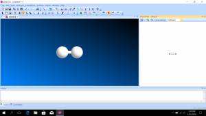
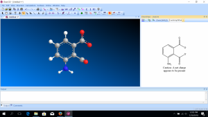
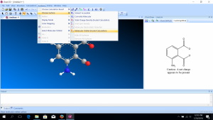
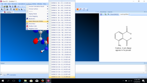
ChemDraw is chemical modeling software. It calculates 3D structures and molecular orbitals, which help chemists predict the chemical and physical properties of theoretical molecules. In this lab, you will use ChemDraw to analyze the structures of molecules in 3D.

Background

This infographic can help you review Lewis dot structures. Note: step 6 is optional and only applies to some molecules. Also note: below step 6 are some tips on when to follow the octet rule and when the octet rule may have an exception.

Procedure

For each given molecule, first, construct a Lewis dot structure as your pre-lab. Then, in lab, make a 3D model in ChemDraw. Using the model in ChemDraw and your textbook, identify the electron geometry or molecular shape of the central atom (if it is not obvious which is the central atom, just pick one of the central atoms). Answer the discussion questions using the models and the software. Complete the worksheet in lab. Hint: consider revising your Lewis dot structure if it disagrees with the 3D model, but trust your brain more than the computer.

To make a molecular model

1. Open Chem3D 15.1
2. Click on the white panel to the right of the main window. It is titled “ChemDraw-LiveLink.”
3. Click on the “A” icon to type, then type the formula of your molecule of interest. For example, you enter H₂O as H2O. When you hit “enter,” the molecule should appear in the big blue window. Note: For more advanced structures or when this method doesn’t produce the structure you were expecting, you will need to type it differently (for example: CH2NH instead of CH3N) or use the tools to draw the molecule by hand. Your instructor and/or TA can show you show you how to do this.
4. Optimize the structure by hitting “control-m.” When you do this, the calculated total energy of the model will appear in an output window.
5. There are several things you can do to get a better look at the molecule.
   1. You can click the third button from the left on the top toolbar to rotate the molecule. It looks like a circle with an arrow on it. After you click it, you can use the mouse to rotate the molecule.
   2. You can click “View” on the main menu, then click “Model Display.” This will present you with many options to change the display of the molecule. For example, “Display Mode” gives you more modes. The “Ball & Stick” mode is most common, but “Wire Frame” is convenient for a very complicated molecule, and “Space Filling” is helpful for visualizing atom size differences.

To measure bond lengths and bond angles on the model

After making the model and optimizing the structure, click “Structure” on the main menu, then “Measurements,” and then select “Generate All Bond Lengths” or “Generate All Bond Angles.”

To measure formal charge of atoms in the model

Hover over the atom of interest. If it has a formal charge, it will say “Formal charge: -1,” for example. It will also display delocalized charges.

To predict the shape of the molecular orbitals

After making the model and optimizing the structure, click “Surfaces” on the main menu, then “Choose Surface,” then “Molecular Orbital.” The HOMO (highest occupied molecular orbital) will automatically be shown, but you can choose another molecular orbital from “Select Molecular Orbital.” You will also see the energies associated with each orbital. The labels are with respect to the HOMO and the LUMO (lowest unoccupied molecular orbital). Notice that the HOMO energy is usually negative, indicating a favorable state, but the LUMO energy is usually positive, indicating an unfavorable state (which is why it is UNOCCUPIED!) The difference between the HOMO and the LUMO energies is called the band gap.

Report

Fill out this worksheet and turn in a paper copy. Optional survey.

Learning Goals

1. Build confidence in yourself as an independent experimentalist;
2. Perform chemical degradation analysis, then use the results to calculate an empirical formula;
3. Use a gravity filtration apparatus;
4. Use a drying oven;
5. Use a Bunsen burner to heat a solid;
6. Observe a redox reaction and a precipitation reaction;
7. Identify sources of uncertainty associated with the procedure and the analytical balance.

Introduction

John Dalton

John Dalton was a chemist, physicist, meterologist, and teacher who lived 1766 – 1844 in England. (Can you believe that he was 34 years old when Middlebury College was founded?!) He was born into a poor Quaker family, so he started supporting himself by working as a teacher at age 12 and continued throughout his life. You can thank Dalton for much of the atomic theory that you are learning in Chem 103.

Over the next two weeks, your laboratory experiments will use Dalton’s atomic theory. In today’s lab, you will determine the molecular formula of a copper compound.

Background

Copper is normally in the 0, +1, or +2 oxidation state. This means copper can combine with 0, 1, or 2 chloride ions. Sometimes water molecules cling to cations and form hydrates. It is difficult to predict the number of water molecules that cling to a salt, but it must always be an integer value.

Today, you will determine the empirical formula of a compound that contains copper, chlorine, and water (Cu_xCl_y zH₂O). You will decompose the compound in order to solve for x, y, and z. The decomposition is in two steps. First, you will heat the compound to dehydrate the compound. Then, you will reduce the copper cations to copper metal to drive off the chlorine. By analyzing how the mass changes after each step, you will be able to solve for the mole ratios in the original compound. A tutorial of this lab is found here.

Procedure

Note: do this lab individually, but share a hood with a “hood mate” and consult with them as needed.

Dry the hydrate

1. 1. Set up a ring stand with a clay triangle on the ring in a fume hood. Place a Bunsen burner underneath with a really small blue flame.
   2. Record the mass of a clean, dry crucible in Table 2.
   3. Place about 1 g of the unknown salt in the crucible. Record the mass of the combined crucible and salt in Table 2. Break up any big chunks with a spatula.
   4. Place your salt and crucible on the clay triangle. Heat super gently. Like giving a baby a warm bath. Stir carefully to prevent burning. Observe the color change from blue-green to brown. If your salt begins to spatter or turn black, lower the heat either by turning down the gas or by raising up your sample from the burner. Don’t hesitate to start over if your salt spatters.
   5. Once the salt is completely brown with no signs of yellow or green, remove the heat and let it cool for about 5 minutes.
   6. Record the mass of the cool crucible containing the dehydrated salt in Table 2. If the mass is not stable, let it cool longer.

Reduce the copper salt to elemental copper

1. Transfer the dehydrated salt to a 50 mL beaker. Rinse the crucible twice with approximately 8 mL of DI H2O each time and pour the rinsate into the same beaker as the dehydrated salt to ensure all of the salt is transferred. Swirl to completely dissolve the salt. Note: the salt turns green when it is dissolved in just a little water, and it turns blue when it is fully hydrated.
2. Coil an approximately 10 cm piece of aluminum wire so that it fits into the beaker. Place it in the beaker and ensure it is completely immersed in the solution. Wait about 30 minutes for the copper to deposit on the surface of the wire. It is finished when the solution is colorless and the bubbling slows. While it is reacting, wash and dry the crucible (but keep yours), set up the next part of the experiment, get a drink of water, work on homework, do your pre-lab for next week (you might want to read through the procedure – it’s a tough one, for sure), go ask Prof. Larrabee questions, call someone in your family, run a 5k, take a nap, etc.
3. Use a spatula to scrape off as much copper as you can from the aluminum wire and put it into the solution.
4. Using that filter paper, set up a funnel filtration apparatus on top of a small Erlenmeyer flask similar to the one shown on the right.
5. Slowly pour the copper and the solution onto the filter paper. Use small amounts of water to rinse all of the copper onto the paper.
6. Open the filter paper, label it, and place it on the watch glass. Put it in the drying oven for about 10 minutes until the copper is dry and crumbly and the paper is dry and begins to brown.
7. When your filter paper starts to brown, carefully transfer all of your copper to your crucible. Put it back in the drying oven for 5 minutes.
8. When you check on your copper, break up the large chunks with a spatula to ensure it is dry throughout. Don’t let it turn black.
9. The drying process is complete when the copper is red/brown and the consistency of Grape Nuts cereal. Let the crucible and copper cool, then weigh it. Record the mass in Table 3. Consult your instructor or TA if the mass of copper is greater than 0.40 g.
10. Pour the filtrate down the drain. Rinse, dry, and return the aluminum wire to where you found it. Save your solid copper!

Oxidize elemental copper to copper oxide

1. Return the copper and crucible to the Bunsen heating set up.

2. Heat the copper and crucible over a hot flame and this time: Burn, baby, BURN. Heat until the copper turns completely black.

3. Let it cool until it is cool enough to handle. Weigh the product. Does the mass increase or decrease? What could cause the mass to increase? What could cause the mass to decrease?

Data analysis

To determine the formula, you will first convert the masses to moles, then divide by the smallest number to get the mole ratios. For example, if you were using a hydrocarbon (composed only of hydrogen and carbon) and you found that it contained 0.25 moles of carbon and 0.99 moles of hydrogen, then you would divide both by 0.25:

0.25 moles carbon / 0.25 = 1 mole carbon

0.99 moles hydrogen / 0.25 = 3.96 moles hydrogen, so approximately 4 moles of hydrogen (remember it must be an integer value!)

Therefore, the empirical formula is CH₄.

Report

Fill out this worksheet. Turn in either a paper or digital copy.

Learning Goals

1. Practice using computational chemistry software;
2. Perform flame tests;
3. Use Erlenmeyer flasks to mix solutions;
4. Use a spectroscope to observe atomic emission;
5. Manipulate units of wavelength and energy;
6. Practice writing ground state and excited state electron configurations.

Background

By Comunicaciones CONICYT – María Teresa Ruiz, Premio Nacional de Ciencias Exactas., CC0, https://commons.wikimedia.org/w/index.php?curid=69688240

María Teresa Ruiz is an astronomer born in 1946. In 1997, Ruiz and coworkers discovered a free-floating brown dwarf, which is an unusual celestial body that is halfway between a planet and a star. She used optical spectroscopy to analyze both the light emitted from the brown dwarf and the light it absorbed. This data gave clues about the brown dwarf’s temperature and chemistry. Over the next two weeks, you will learn about optical spectroscopy, both emission and absorption.

Colored chemicals absorb and/or emit light in the visible portion of the electromagnetic spectrum, which has a wavelength of approximately 400 – 700 nm. The color of the absorbed or emitted light depends on the amount of energy the chemical absorbed or emitted. Wavelength and energy are negatively correlated. 

Absorption occurs when an electron in a chemical absorbs energy from the light, temporarily promoting the electron to a higher energy orbital. Light emission can occur when an electron relaxes back to the ground state and produces light, but emission is less common than absorption because there are many of non-radiative ways for the electron to relax. 

Most chemicals are colored because they absorb light and reflect only a portion of incident light. In this case, the color that a chemical absorbs is the opposite of the color that it appears. The color wheel shows you which colors are opposite of one another. The color wheel helps you to predict the color that a chemical absorbs based on the color it appears (and vice versa). For example, beta-carotene, a pigment found in many fruits and vegetables including carrots, absorbs purple and blue light (400 – 500 nm) and reflects all of the other colors, so it appears yellow/orange. It DOES NOT emit yellow/orange light.

If a chemical is colored due to emission, then the color it appears corresponds to the color it emits. Many processes can temporarily promote an electron to a higher energy orbital and induce emission; these include light, heat, electricity, and chemical reactions. Today, you will observe light emission from electricity in part 1, chemical reactions in part 2, and heat in part 3.

Objective

In part 1 of this lab, you will observe emission of atomic hydrogen which will be excited with electricity. Using the Rydberg formula, you should be able to figure out which lines in the emission correspond to which transitions in the hydrogen atom. Refer to Chapter 3.1 in your textbook to refresh yourself on the Rydberg formula. You will also model molecular hydrogen to better understand molecular orbital theory.

In part 2 of this lab, you will observe the emission from a light-producing chemical reaction. You will model the product and run calculations to determine the quantum mechanical source of the emission.

In part 3 of this lab, you will perform flame tests and propose the chemicals you could use to make a fireworks display.

You may perform parts 1, 2, and 3 in any order.

Procedure

Part 1: Hydrogen

Experimental component

Note: perform this section individually.

1. First, look through the spectroscope through the window. You should see a rainbow approximately spanning 4.0 – 8.0 on the scale in the spectroscope. The units on these instruments are in hundreds of nanometers, so 4.0 corresponds to 4.0 x 10² nanometers. If you don’t see a rainbow across this range, ask your TA or instructor for help.
2. Turn on the hydrogen lamp and observe the emission through the spectroscope.
3. Use the Rydberg formula to calculate the energy transition associated with each line. h = 6.626*10^-34 Js, c = 2.9979*10⁸ m/s
4. Turn off light source once you are finished observing the emission. Record your observations.
5. Extra lamps are provided for you to explore, but they are not required for this lab.

Computational component

1. Open Chem3D 18.0
2. Click on the white panel to the right of the main window. It is titled “ChemDraw-LiveLink.”
3. In the text bar, type “Hydrogen,” then hit “enter.” A molecule should appear.
4. Optimize the structure by hitting “control-m.”
5. There are several things you can do to get a better look at the molecule.
   • You can click the third button from the left on the top toolbar to rotate the molecule. It looks like a circle with an arrow on it. After you click it, you can use the mouse to rotate the molecule.
   • You can click “View” on the main menu, then click “Model Display.” This will present you with many options to change the display of the molecule. For example, “Display Mode” gives you more modes. The “Ball & Stick” mode is most common, but “Wire Frame” is convenient for a very complicated molecule, and “Space Filling” is helpful for visualizing atom size differences.
6. After making the model and optimizing the structure, click “Surfaces” on the main menu, then “Choose Surface,” then “Molecular Orbital.”
7. The HOMO (highest occupied molecular orbital) will automatically be shown, but you can choose another molecular orbital from “Select Molecular Orbital.” You will also see the energies associated with each orbital. The labels are with respect to the HOMO and the LUMO (lowest unoccupied molecular orbital). Notice that the HOMO energy is usually negative, indicating a favorable state, but the LUMO energy is usually positive, indicating an unfavorable state (which is why it is UNOCCUPIED!)
8. Draw on your worksheet the HOMO and the LUMO. Indicate color differences either by using color in your drawing or by shading.

Part 2: Luminol

Experimental component

Source: https://www.carolina.com/teacher-resources/Interactive/luminol-glowing-reaction/tr10786.tr

Note: perform this section with a partner.

Create Solution A

1. Measure out the correct mass of NaOH pellets according to your pre-lab calculation. Place into a 250 or 300 mL Erlenmeyer flask.
2. Measure out 100 mL of DI water in a 150 mL beaker. Add to the Erlenmeyer flask with the NaOH pellets. Swirl to dissolve.
3. Measure out ~0.18 g of luminol in a weigh boat. Add to the Erlenmeyer flask. Swirl to dissolve. Pro-tip: an Erlenmeyer flask is a great choice when mixing up a solution from a solid because you can swirl without the solution splashing out of the flask. Always use an Erlenmeyer flask that has plenty of extra space to allow you to swirl.
4. Record the appearance of Solution A.

Create Solution B

1. Measure out 0.03 g of potassium ferricyanide.
2. In a second 250  or 300 mL Erlenmeyer flask, add 100 mL of DI water, 1 mL of 3% hydrogen peroxide, and the 0.03 g of potassium ferricyanide. Swirl to dissolve.

Mix them together

1. Go into the dark room.
2. Slowly pour the two solutions simultaneously into the funnel at the top of the apparatus.
3. Record your observations immediately after the two solutions mix.
4. Dispose of the solution in the waste containers.

Computational component

1. Open Chem3D 18.0
2. Click on the white panel to the right of the main window. It is titled “ChemDraw-LiveLink.”
3. In the text bar, type “3-aminophthalate,” then hit “enter.” A molecule should appear.
4. Optimize the structure by hitting “control-m.”
5. After making the model, click “Surfaces” on the main menu, then “Choose Surface,” then “Molecular Orbital.”
6. The HOMO (highest occupied molecular orbital) will automatically be shown, but you can choose another molecular orbital from “Select Molecular Orbital.” You will also see the energies associated with each orbital. The labels are with respect to the HOMO and the LUMO (lowest unoccupied molecular orbital).
7. You will need to record the difference between the MOs prescribed on your worksheet. Note that ChemDraw reports the band gap in terms of eV, so you will need to convert from those energy units to wavelength units to determine the color that corresponds to each of these potential transitions. This will require using Plank’s constant in different units than you typically use: h = 4.1357 × 10^–15 eV s. I suggest that you use Excel or some other software to do this repeated calculation. Once you know the colors of each possible transition, you will be able to choose the most likely transition that corresponds to the color you observed.

Part 3: Flame tests

Note: perform this section individually in a fume hood.

1. Observe sources one at a time by eye. If you are color-blind, you will need to work with a non-color-blind partner.
2. Light a bunsen burner with a non-luminous blue flame using your amber tubing and your bunsen burner in  a fume hood.
3. For the first metal, obtain a wooden splint that has been soaked in the metal solution.
4. Wave the wet part of the splint in the hottest part of the flame (the top of the inner cone).
5. The color you observe is the first color you see, not the yellow color of the wood burning. If you aren’t sure what color is wood burning, experiment by burning a dry splint.
6. Write down your observations of the color(s) and intensity on your worksheet.

Report

Fill out this worksheet. Turn in either a paper or digital copy.

Learning goals: maintain safety in a chemistry laboratory,  follow instructions to complete a laboratory experiment, collect experimental data, explain likely sources of experimental error

Introduction

A chemical reaction occurs when electrons and/or bonds rearrange. A chemical reaction can be described with a chemical equation. You may notice a chemical reaction has occurred by one of the following indicators:

• A color change (eg. a colorless solution turns red),
• A change of state (eg. a solid precipitates in a solution),
• A change in temperature (eg. a solution gets hot).

Today’s lab activity is an example of a chemical reaction. You will form a golden solid from two colorless solids.

Background

Lead nitrate and potassium iodide are both highly soluble in water. This means:
Pb(NO₃)_{2 (s)} → Pb²⁺_(aq) + 2NO₃^–_(aq)
KI_(s) → K⁺_(aq) + I^–_(aq)

When you mix those two solutions together, all four ions encounter each other, and that’s when the chemical reaction occurs:

Pb²⁺_(aq) + 2I^–_(aq) → PbI_2(s)

The potassium and nitrate ions are not involved in the chemical reaction; they are called “spectator ions.” They are present in the same amounts before and after the reaction (on both sides of the arrow).

Pb²⁺_(aq) + 2NO₃^–_(aq) + 2K⁺_(aq) + 2I^–_(aq) → PbI_2(s) + 2NO₃^–_(aq) + 2K⁺_(aq)

When the solid forms, it first looks like yellow clouds because the tiny solid particles are suspended in the solution (like mud). We have to take advantage of its slight solubility in order to form a sparkling, golden solid. When you first add the lead nitrate to the potassium iodide, you will notice the cloudy precipitate forms and then dissolves. This is because lead nitrate is “slightly soluble.” 0.08 g of it can dissolve in 100 mL of water: the yellow clouds only remain visible when there is more than 80 mg present per 100 mL of water.

Temperature dependence of solubility for several solids. Source: http://wps.prenhall.com

Many solids are more soluble in hot water than cold. Heating the solution will cause the lead nitrate to dissolve completely so that it can slowly crystallize as it cools, which forms large crystals.

Procedure

Note: do this lab individually.

Prepare solutions

1. Tare a 250 or 300 mL Erlenmeyer flask labeled “lead nitrate”. Add approximately 0.3 g of lead nitrate to the flask. Record the exact mass on the worksheet.
2. Measure out 100 mL of deionized water (DI H2O) with a graduated cylinder. Pour the water into the flask containing the solid lead nitrate. Swirl to dissolve.
3. Repeat this procedure with another flask for the Potassium Iodide.
4. Add a few drops of 0.5 M hydrochloric acid to each solution.

Form Crystalline Lead Iodide

1. Add the lead nitrate to the potassium iodide one drop at a time, swirling to dissolve after each drop. How many drops can dissolve? Once the yellow clouds start to form and will not dissolve when swirling, pour in the remainder of the lead nitrate. Record your observations.
2. Prepare a hot water bath with a Bunsen burner, a ring stand, a ring, a wire mesh, and an 800 mL or 1000 mL beaker – similar to the picture to the right. Alternatively, you can use a tripod instead of the ring stand and ring. Put approximately 500 mL of water in the beaker, then heat the water up to boiling. (Hint: If you read through these instructions before coming to lab, you will probably start with this step so you do not have to wait for your water to heat up.)
3. Carefully place the Erlenmeyer flask containing the lead iodide in the hot water bath. Heat the lead iodide solution up to about 80^oC or until the lead iodide dissolves. Record your observations.
4. Once the lead iodide has completely dissolved, remove the Erlenmeyer flask from the hot water bath. Set it on the bench top and watch the crystals form. Wait about half an hour for the crystals to precipitate slowly at room temperature. (The longer you wait, the nicer your crystals will look.) Record your observations. This may take a few minutes, so while you’re waiting, you should work on cleaning up the hot water bath, completing the worksheet, inventorying your glassware, and preparing for the next steps:
   • Prepare an ice bath. With the same 800 mL beaker, fill it about halfway with ice and water.
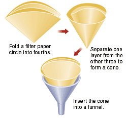
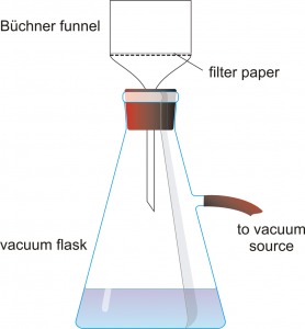
   • Obtain a Büchner funnel, a filter flask, and an appropriately sized piece of filter paper. Record the mass of the filter paper.
   • Set up a filter system like the one shown to the left. Wet the filter paper with a few mLs of water so that it sticks to the bottom of the funnel.
5. After you have waited about half an hour, put the flask into the ice bath for about ten minutes.
6. After that, turn on the vacuum source and pour the crystals and solution into the Büchner funnel. Use a few mLs of ice water to rinse away any crystals that may have stuck to the sides of the flask.
7. Turn off the vacuum source once the crystals and paper appear dry.
8. Weigh the filter paper and crystals on a tared watch glass. Record the mass on your worksheet and calculate the final mass of crystals.
9. Ask your instructor or TA to check your data and observations before you clean up or leave.

Clean up

Pour the filtrate into the waste beaker labeled “lead iodide waste liquid.” Take a picture of your pretty crystals to show your roommate, then put the crystals and filter paper into the waste beaker labeled “solid lead iodide waste.” Pour hot water and ice baths down the sink. Rinse all glassware and return to them to where you found them.

Report

Complete the worksheet. Turn in either a paper or digital copy. This article will help you with the conclusion question. Optional survey.