
Learning Goals
- Practice using computational chemistry software;
- Perform flame tests;
- Use Erlenmeyer flasks to mix solutions;
- Use a spectroscope to observe atomic emission;
- Manipulate units of wavelength and energy;
- Practice writing ground state and excited state electron configurations.
Background

By Comunicaciones CONICYT – María Teresa Ruiz, Premio Nacional de Ciencias Exactas., CC0, https://commons.wikimedia.org/w/index.php?curid=69688240
María Teresa Ruiz is an astronomer born in 1946. In 1997, Ruiz and coworkers discovered a free-floating brown dwarf, which is an unusual celestial body that is halfway between a planet and a star. She used optical spectroscopy to analyze both the light emitted from the brown dwarf and the light it absorbed. This data gave clues about the brown dwarf’s temperature and chemistry. Over the next two weeks, you will learn about optical spectroscopy, both emission and absorption.
Colored chemicals absorb and/or emit light in the visible portion of the electromagnetic spectrum, which has a wavelength of approximately 400 – 700 nm. The color of the absorbed or emitted light depends on the amount of energy the chemical absorbed or emitted. Wavelength and energy are negatively correlated.
Absorption occurs when an electron in a chemical absorbs energy from the light, temporarily promoting the electron to a higher energy orbital. Light emission can occur when an electron relaxes back to the ground state and produces light, but emission is less common than absorption because there are many of non-radiative ways for the electron to relax. 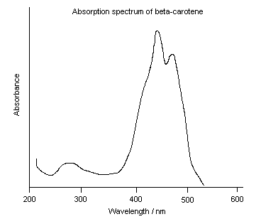
Most chemicals are colored because they absorb light and reflect only a portion of incident light. In this case, the color that a chemical absorbs is the opposite of the color that it appears. The color wheel shows you which colors are opposite of one another. The color wheel helps you to predict the color that a chemical absorbs based on the color it appears (and vice versa). For example, beta-carotene, a pigment found in many fruits and vegetables including carrots, absorbs purple and blue light (400 – 500 nm) and reflects all of the other colors, so it appears yellow/orange. It DOES NOT emit yellow/orange light.
If a chemical is colored due to emission, then the color it appears corresponds to the color it emits. Many processes can temporarily promote an electron to a higher energy orbital and induce emission; these include light, heat, electricity, and chemical reactions. Today, you will observe light emission from electricity in part 1, chemical reactions in part 2, and heat in part 3.
Objective
In part 1 of this lab, you will observe emission of atomic hydrogen which will be excited with electricity. Using the Rydberg formula, you should be able to figure out which lines in the emission correspond to which transitions in the hydrogen atom. Refer to Chapter 3.1 in your textbook to refresh yourself on the Rydberg formula. You will also model molecular hydrogen to better understand molecular orbital theory.
In part 2 of this lab, you will observe the emission from a light-producing chemical reaction. You will model the product and run calculations to determine the quantum mechanical source of the emission.
In part 3 of this lab, you will perform flame tests and propose the chemicals you could use to make a fireworks display.
You may perform parts 1, 2, and 3 in any order.
Procedure
Part 1: Hydrogen
Experimental component
Note: perform this section individually.
- First, look through the spectroscope through the window. You should see a rainbow approximately spanning 4.0 – 8.0 on the scale in the spectroscope. The units on these instruments are in hundreds of nanometers, so 4.0 corresponds to 4.0 x 10² nanometers. If you don’t see a rainbow across this range, ask your TA or instructor for help.
- Turn on the hydrogen lamp and observe the emission through the spectroscope.
- Use the Rydberg formula to calculate the energy transition associated with each line. h = 6.626*10-34 Js, c = 2.9979*108 m/s
- Turn off light source once you are finished observing the emission. Record your observations.
- Extra lamps are provided for you to explore, but they are not required for this lab.
Computational component
- Open Chem3D 18.0
- Click on the white panel to the right of the main window. It is titled “ChemDraw-LiveLink.”
- In the text bar, type “Hydrogen,” then hit “enter.” A molecule should appear.

- Optimize the structure by hitting “control-m.”
- There are several things you can do to get a better look at the molecule.
- You can click the third button from the left on the top toolbar to rotate the molecule. It looks like a circle with an arrow on it. After you click it, you can use the mouse to rotate the molecule.
- You can click “View” on the main menu, then click “Model Display.” This will present you with many options to change the display of the molecule. For example, “Display Mode” gives you more modes. The “Ball & Stick” mode is most common, but “Wire Frame” is convenient for a very complicated molecule, and “Space Filling” is helpful for visualizing atom size differences.
- After making the model and optimizing the structure, click “Surfaces” on the main menu, then “Choose Surface,” then “Molecular Orbital.”

- The HOMO (highest occupied molecular orbital) will automatically be shown, but you can choose another molecular orbital from “Select Molecular Orbital.” You will also see the energies associated with each orbital. The labels are with respect to the HOMO and the LUMO (lowest unoccupied molecular orbital). Notice that the HOMO energy is usually negative, indicating a favorable state, but the LUMO energy is usually positive, indicating an unfavorable state (which is why it is UNOCCUPIED!)
- Draw on your worksheet the HOMO and the LUMO. Indicate color differences either by using color in your drawing or by shading.
Part 2: Luminol
Experimental component
Source: https://www.carolina.com/teacher-resources/Interactive/luminol-glowing-reaction/tr10786.tr
Note: perform this section with a partner.
Create Solution A
- Measure out the correct mass of NaOH pellets according to your pre-lab calculation. Place into a 250 or 300 mL Erlenmeyer flask.
- Measure out 100 mL of DI water in a 150 mL beaker. Add to the Erlenmeyer flask with the NaOH pellets. Swirl to dissolve.
- Measure out ~0.18 g of luminol in a weigh boat. Add to the Erlenmeyer flask. Swirl to dissolve. Pro-tip: an Erlenmeyer flask is a great choice when mixing up a solution from a solid because you can swirl without the solution splashing out of the flask. Always use an Erlenmeyer flask that has plenty of extra space to allow you to swirl.
- Record the appearance of Solution A.
Create Solution B
- Measure out 0.03 g of potassium ferricyanide.
- In a second 250 or 300 mL Erlenmeyer flask, add 100 mL of DI water, 1 mL of 3% hydrogen peroxide, and the 0.03 g of potassium ferricyanide. Swirl to dissolve.
Mix them together
- Go into the dark room.
- Slowly pour the two solutions simultaneously into the funnel at the top of the apparatus.
- Record your observations immediately after the two solutions mix.
- Dispose of the solution in the waste containers.
Computational component
- Open Chem3D 18.0
- Click on the white panel to the right of the main window. It is titled “ChemDraw-LiveLink.”
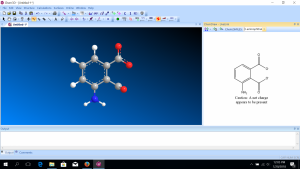
- In the text bar, type “3-aminophthalate,” then hit “enter.” A molecule should appear.
- Optimize the structure by hitting “control-m.”
- After making the model, click “Surfaces” on the main menu, then “Choose Surface,” then “Molecular Orbital.”
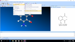
- The HOMO (highest occupied molecular orbital) will automatically be shown, but you can choose another molecular orbital from “Select Molecular Orbital.” You will also see the energies associated with each orbital. The labels are with respect to the HOMO and the LUMO (lowest unoccupied molecular orbital).
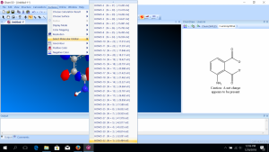
- You will need to record the difference between the MOs prescribed on your worksheet. Note that ChemDraw reports the band gap in terms of eV, so you will need to convert from those energy units to wavelength units to determine the color that corresponds to each of these potential transitions. This will require using Plank’s constant in different units than you typically use: h = 4.1357 × 10⁻¹⁵ eV s. I suggest that you use Excel or some other software to do this repeated calculation. Once you know the colors of each possible transition, you will be able to choose the most likely transition that corresponds to the color you observed.
Part 3: Flame tests
Note: perform this section individually in a fume hood.
- Observe sources one at a time by eye. If you are color-blind, you will need to work with a non-color-blind partner.
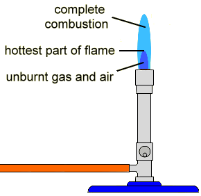
- Light a bunsen burner with a non-luminous blue flame using your amber tubing and your bunsen burner in a fume hood.
- For the first metal, obtain a wooden splint that has been soaked in the metal solution.
- Wave the wet part of the splint in the hottest part of the flame (the top of the inner cone).
- The color you observe is the first color you see, not the yellow color of the wood burning. If you aren’t sure what color is wood burning, experiment by burning a dry splint.
- Write down your observations of the color(s) and intensity on your worksheet.
Report
Fill out this worksheet. Turn in either a paper or digital copy.
 Obtain a Büchner funnel, a filter flask, and an appropriately sized piece of filter paper. Record the mass of the filter paper.